Last year, Excel released some updates including the unveiling of XLOOKUP as well as XMATCH. In this post, I’ll show you how to use the XMATCH function and also why you may not have a need for it.
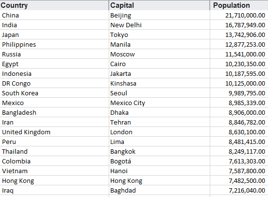
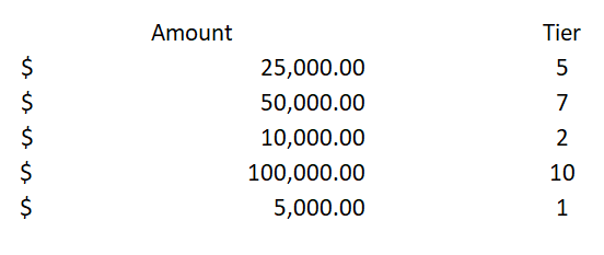
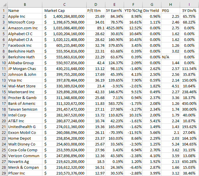
For this example, I’m going to use a list of the stocks with the largest market caps on the U.S. exchanges as of Feb.7, 2020. Here’s what my data looks like:
XMATCH can achieve the same results as MATCH does when looking for data, but if you wanted the same functionality you could just use MATCH. Instead, let’s start by looking at some of the other things that Microsoft claims XMATCH can do.
XMATCH is not a suitable COUNTIF replacement
One of the things that XMATCH can supposedly do is when you’re looking up numbers, it will count the number of times that values fall above or below a threshold. For this example, we will look at the number of stocks on this list with market caps of more than $1 trillion.
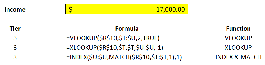
To do this, you would use $1,000,000,000,000 as your lookup value and set the third argument of the function, called match mode, to 1, which looks at an exact match or the next larger item. Here’s how the formula looks like:
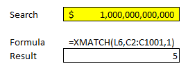
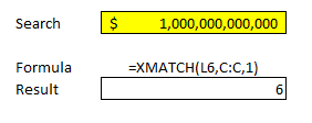
Where L6 is the cell that has the number that XMATCH will search for (1,000,000). This formula correctly gives me five matches that are more than $1 trillion that appear on the list. However, if I include the header, the results change:
This leads me to believe that it’s still looking for the closest match and not really counting the number of values that meet the criteria. And indeed, when I changed some of the market cap numbers so that they were more than $1 trillion, XMATCH didn’t compute them correctly since they weren’t in descending order. I’m assuming what Microsoft is implying with XMATCH is that if your data is sorted in ascending order, it would be able to tell you where the smallest value is that meets your criteria. For example, The sixth row in the data set was $1.02 trillion and that was the lowest entry that was more than $1 trillion. Technically, if the data was in descending order then everything above that will be more than $1 trillion.
However, that’s very different from actually counting the numbers over that threshold. And that’s why COUNTIF is still vastly superior to XMATCH. Here’s how the two functions worked when I added four additional entries (not in order) of more than $1 trillion, bringing my tally to nine:
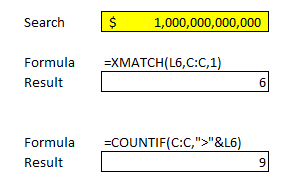
In the COUNTIF function, it still correctly counted nine instances where there was more than $1 trillion on the list. XMATCH, meanwhile, continued to point to the sixth row.
These issues are confirmed when we look at the number of values below $1 trillion:
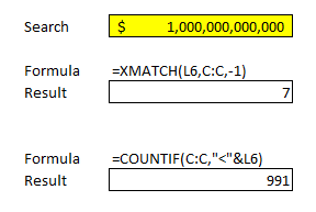
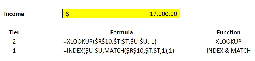
The -1 argument in match mode is the opposite of 1, and it looks at the exact match or next smaller item. However, the results, as you can see, were very different and not what I would have expected. It appeared to point me to the closest number to $1 trillion without going over. COUNTIF, meanwhile, continued to correctly count the number of items that were below $1 trillion. And with 1,000 items in my data set, it makes sense that 991 were below if nine were above the threshold. Unfortunately, that same logic doesn’t work with XMATCH.
As a replacement for COUNTIF, XMATCH gets a fail as it’s clear that it’s not really counting the number of instances. Only under very specific circumstances would the function do that, such as if the data was in descending order. And even then, you’d still need to do a calculation for the header or if you’re looking at the number of items below a threshold. It’s more trouble than it’s worth and COUNTIF has the benefit of also being available in older versions of Excel, even going back to Excel 2000. That’s important if you’ll ever need to work on an older version of Excel.
Using XMATCH to search for text is not any better than using MATCH
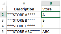
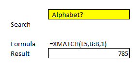
If you’re using XMATCH for matching text, it won’t be able to count the instances but you can use it to find the first instance of it. Some companies trade under multiple tickers and you’ll notice Google’s parent company Alphabet shows up twice in this list. Here’s what happens when I try to use the XMATCH function to find the first instance:
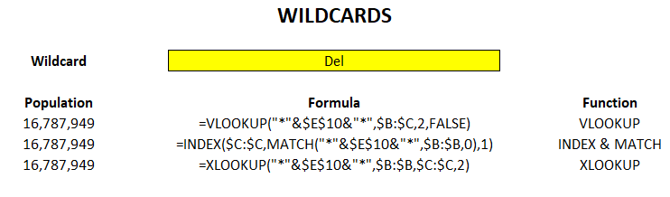
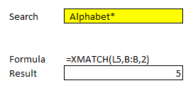
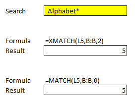
I’m using a question mark after the text as that’s what Microsoft instructs users to do when looking for partial matches. However, if I ignore that advice and use an asterisk and specify I’m using a wildcard match, then it appears to fix the issue:
You may be wondering how the regular MATCH function did:
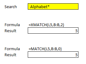
Besides changing the last argument, the functions are nearly identical in how they’re used to find partial matches.
Let’s compare how the functions work when we’re looking at exact matches. For this example, I renamed the multiple Alphabet names so that they only spell out Alphabet with no mention of share classes, e.g. so they’re exactly the same. Here’s how XMATCH does on a simple match calculation:
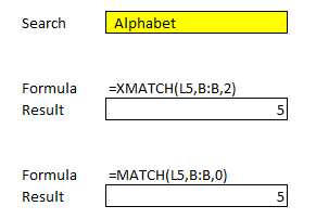
Here again, there’s little distinction between the two functions.
Microsoft also advertises that XMATCH can be used in an INDEX/MATCH combination, but even that seems kind of pointless.
Using XMATCH with INDEX makes little sense
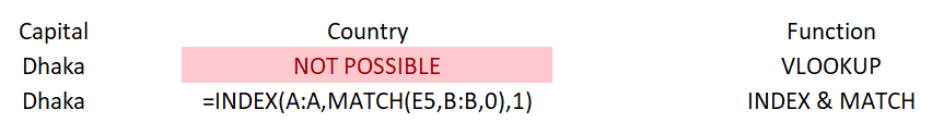
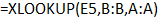
Let’s use these functions to grab the intersect between the company name and its dividend yield. The name is in column B while the dividend yield is in column G. All the headers are in the first row. Here’s how the formula looks like with the use of XMATCH:
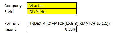
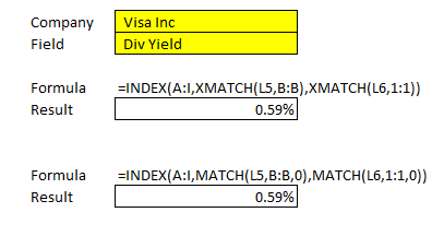
In this example, XMATCH correctly pulled the right percentage for Visa’s dividend yield of 0.59%.
That would be really, really cool if the MATCH function didn’t already do the exact same thing. By getting rid of the X in the XMATCH function, thus making it just a MATCH function, and adding a 0 for the third argument, I get the same exact result:
XMATCH doesn’t improve upon anything when it involves the INDEX and MATCH combination. We’re talking a slight change to the syntax, that’s about it. And again, from a functionality point of view, there’s just no reason to swap a new function in when the existing one works just as well, especially since there’s no backwards compatibility on older versions of Excel for XMATCH.
What XMATCH can do well
Everything that the MATCH function can do, XMATCH can do as well. That’s the good news. There is, however, one thing that XMATCH can do better, and that’s look for data in the reverse order. Here’s a simple example of how both functions work when we’re looking for the first value that contains the word Alphabet:
Both functions correctly yield the same results. Again, the change here is mainly to do with syntax. Under the new XMATCH, if I set the third argument (match mode) to 0 and look for an exact match, I’ll get an error. But if I set it to 2, which is wildcard character match, it will produce the correct result: Alphabet, which first shows up on the fifth row. However, it’s easy to see how this will confuse users who are familiar with MATCH and just use 0 for the third argument, which will also produce the correct result in this case. This is another example of where the syntax has gotten more complicated and not given the user any additional advantage.
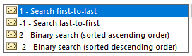
The one exception to that, however, is if you want to do a search in the reverse order. MATCH currently will go from the first row and work its way down. Once there’s a match, it will stop there. Here’s how the XMATCH function performs when we’re doing a last-to-first search, as indicated in the fourth argument where the value is -1:
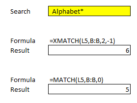
This time XMATCH does correctly pull the sixth row, which is where Alphabet would first show up if we were looking from the bottom and moving up. MATCH, unfortunately, doesn’t have the option to do that and a user would have to rearrange their data to get the same result.
The reverse-order search is the only advantage I can see from testing out XMATCH. Unfortunately, the new function doesn’t add anything significantly new and at worse, it can lead to incorrect results, especially if you’re planning to use it to replace COUNTIF.
Why learning new functions may not be worthwhile, at least not initially
It’s possible that in future updates the XMATCH function will work better but for now, there’s not a whole lot of reason to use it. One of the biggest disadvantages of new functions is that they won’t be helpful to you if you’re working on an older file. It’s not uncommon for people to be working on Excel versions that are more than 10 years old. Not everyone needs the latest-and-greatest version, and mastering a new function may not prove to be worthwhile, especially when older functions work just as well, if not better.
If you liked this post on how to use XMATCH, please give this site a like on Facebook and also be sure to check out some of the many templates that we have available for download. You can also follow us on Twitter and YouTube.