H2EPostDropDowns

Create an Excel Drop Down List Without Blanks

In a previous post, I covered how to create a form in Excel. Although I didn’t go over drop down lists specifically, they are one element you could incorporate into them. The problem is that your list can change over time, getting bigger or smaller. And that can make it difficult to maintain if your list isn’t dynamic as it will involve you always having to manually change the range of your drop down list. Otherwise, it could be incomplete or contain blanks. Below, I’ll show you how you can manually change your drop down list in excel and create it without blanks while also making it dynamic so that you don’t need to worry about whether it changes over time.

Setting up the drop down list

First, let’s start with the basics — creating the list. To create a drop down list in Excel, you just need a series of options to choose from. My list is going to be made up of the top 30 places to visit. I’m just going to put those names in a list.

After entering in the list of places into Excel, the next thing I will do is select all the values, and create a named range. This is as simple as just entering a value next to the formula bar, where you see the cell location. I will call this range VacationSpots:
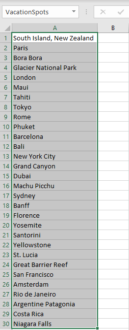
Named range in Excel containing popular vacation spots.

There is no need to add headers or anything else. Just select the values, enter in a name for the list, and hit enter. A longer approach would be to go to the Formula tab and select Name Manager:
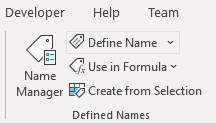
Name Manager in Excel.

Clicking this will show you all of the named ranges in the workbook:
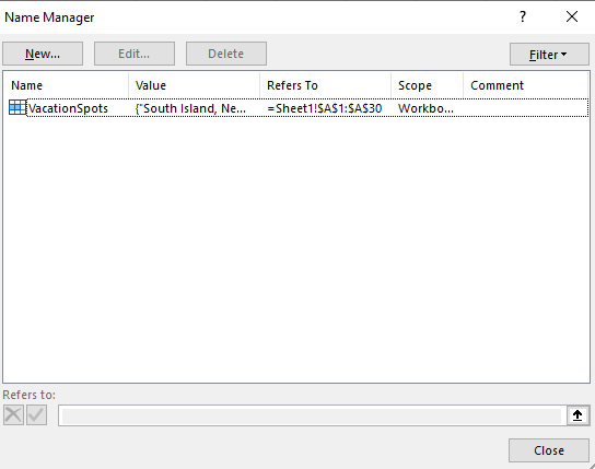
Name manager showing a list of all the named ranges in an Excel workbook.

It shows you the named range I created. However, I could also create one from this screen and also Edit my existing range. This is where you would go to make the change manually. Clicking on the Edit button would give you this screen:
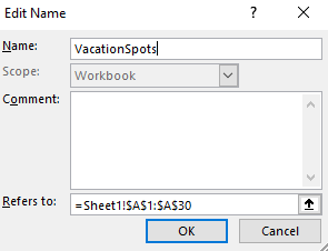
Editing a named range in Excel.

As you can, here I can manually change the address as needed in case the list changes. However, this is obviously not optimal as it can be a tedious process if your list changes frequently.

Creating the drop down

Now that my list has been created, I can set up the actual drop down. To do this, I’m going to select a cell and under the Data tab, click on Data Validation. Here, there is a place to enter your list of values:
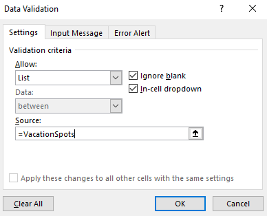
Entering in data validation in Excel.

Under the Allow section, I choose List. And for the Source, I enter the ‘=’ sign followed by my named range, VacationSpots. Now, when I click OK and go to the cell that contains the data validation, this is what I see when I select it:

Cell showing a drop down arrow.

Clicking on the drop down arrow will show me my list of options, in the same order that they appear in my list:
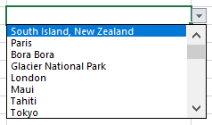
Selecting from a list of drop down options in Excel.

I can select any of the values and my cell will update accordingly. This is great, but what if I decided to add more items to my list, perhaps 10 or 20 more locations I want to visit? Next, I’ll go the different ways you can create drop down lists in Excel without blanks.

Option 1: Create extra spaces in your drop down list at the very end

Technically this step involves blank spaces, which is not what this post is supposed to be about. However, I just wanted to show you how this could work. If your list has dozens of items, then having extra blanks may not be that big of a deal. For example, say I edit my named range so that it goes to 50 rows. If you do that and include empty cells, this is the biggest problem you’ll face:
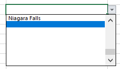
Empty values in a drop down list.

My list no longer starts from the top, it goes to the first blank cell. This can be an annoying problem because now it looks like all of my options aren’t there (they are, but I have to scroll up every time). This is probably the main reason people want to avoid having blank values in their lists. If the blank values simply came after all of your selections, that might be more tolerable. But because they impact where your drop down list begins from, it can be a nuisance.

The good news is there is a simple way to get around this. For all your empty cells, enter just a single empty character. Select a cell, hit the space bar, get out of the cell, and copy that value down. Now, your empty cells technically aren’t empty because they contain a space. And by doing so, the drop down list now starts from the top again. You will still have blank values, but this time they will show at the bottom of your drop down list:
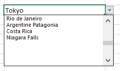
Drop down list with blanks at the bottom.

If this is acceptable then you can stop here. If you are still intent on getting rid of any possible blank value whatsoever, then head over to the next option.

Option 2: Creating a table to create a nonblank list

This option is the easiest method for getting rid of blank values. What you need to do here is convert your list into a table. Select a cell on your list, click on the Insert tab and then click Table:

Creating a table in Excel.

Leave the option for headers unchecked and then click OK. You should see something like this:

Newly created table in Excel.

By default, Excel will apply its formatting and design but you can change the look of it to make it blend in more with your spreadsheet. You can also re-name the header from Column1. Either way, you can now create a new drop down list from this table. Since the values are in range A2:A31 in my spreadsheet, that is what I will enter for my new Data Validation list:
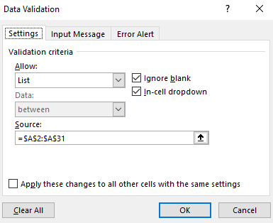
Data validation list in Excel.

You can either select the range, or enter it in yourself. But if you enter it, you need to include the $ signs otherwise it will not auto-update properly. Now, I’ll go to my list add ‘New City’ to the bottom of the table. When I do that, the table automatically expands which you can notice because I haven’t changed the design and so the colors change:

Table in Excel after adding a new value.

And if I go back to the Data Validation settings, my source has automatically been updated:
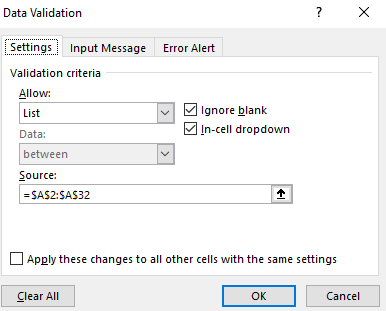
Data validation list in Excel updated.

This is a really easy way to make your drop-down list automatically update without the need for any formulas.

If the table you are referencing isn’t on the same sheet as your drop-down list, then you will need to use the INDIRECT function reference it. For instance, if you have created a table called Table1 (which should contain just one column for your list) on a different sheet, you can reference it the following way:
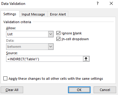
This will allow you to reference the list even if it is on a different sheet.

Option 3: Using a formula to remove the blanks in your drop down list

If for whatever reason creating a table isn’t an option for you, you can still create a dynamic list using a formula. Here, I’ll go back to creating a named range. Except rather than selecting a fixed set of cells, I will rely on a single formula. First, I’ll go back to the Name Manger. I’ll create a new named range. The formula for this can look a bit complex so I will break it down into parts.

First, I’m going to use the OFFSET function. This is because it can allow me to specify a height and width, which is crucial to making this work. My data starts in cell A1, and that’s where my formula will begin:

=OFFSET(A1,0,0

A1 is my starting point and that is the first argument. The next two arguments are whether I want to offset and move to any adjacent rows or columns. Since I don’t, I leave those values as zeros. It is the next argument that is critical, as it relates to the height. Here is where I will use a COUNTA function. I want to count the number of nonblank values in my list. My formula looks as follows:

=COUNTA(A:A)

I will embed this within my previous formula:

=OFFSET(A1,0,0,COUNTA(A:A)

For the width, I will set the last argument to 1, since I don’t want to include any extra columns. Here is my completed formula:
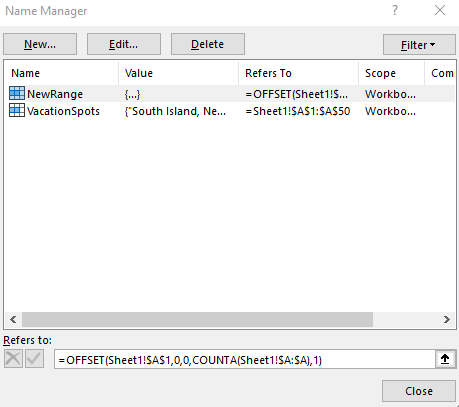
Named range in Excel using the Offset function.

You always want to used $ signs in named ranges so that they don’t move on you. Now that this is set up, I can use this NewRange as my Data Validation source. And just like with a table, whether the list gets bigger or smaller, my named range and the drop down list will automatically update.

However, what if your list contains some formulas that look blank but really aren’t? Formulas are a great example of cells that can look empty even if they aren’t. The COUNTA function will count these values and you could again be back to square one with additional blank values. One way you can get around this is by counting the cells that are blanks, and subtracting that from the total rows. The formula would look as follows:

=ROWS(A:A)-COUNTIF(A:A,””)

Using this, you should correctly arrive at the number of cells that contain text and that aren’t blank as a result of a formula You can then insert that formula in your named range, in place of the COUNTA formula:
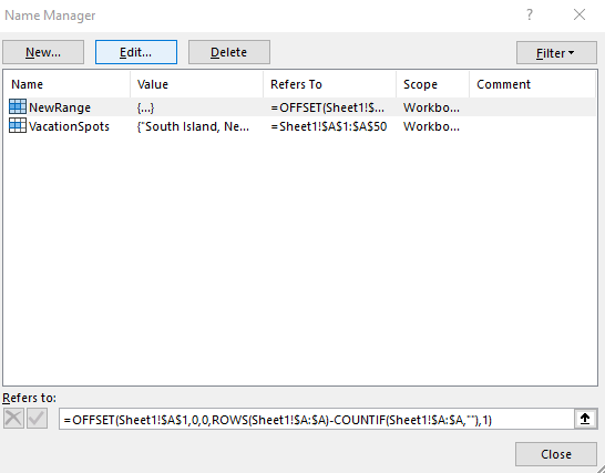
Named range in Excel using the countif and offset formula.

As you can see, this method isn’t the easiest and that is why I left it for the end. However, there are multiple different ways you can create a drop down list in excel without blanks. But it’s important because by removing blanks, it will make your form or spreadsheet look more polished by not having blank values in them.


If you liked this post on how to create a drop down list in Excel without blanks, please give this site a like on Facebook and also be sure to check out some of the many templates that we have available for download. You can also follow us on Twitter and YouTube.

movingaverage

How to Do a Moving Average in Excel

If you’re doing any type of data analysis, a moving average can be useful in smoothing trends and normalizing data. Below, I’ll show you how you can easily create a moving average in Excel. The data will again be based on the retail and food services sales data that I used in my post covering how to transpose data.

With the data now converted from the summary table, it’s in the right format for analyzing and averaging the data.

Calculating an average

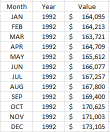
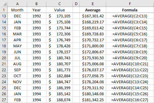
To calculate an average in Excel, all you need to do is use the AVERAGE function. Simply select the range that you want to average, and the function will take care of the calculation for you. Here’s an excerpt from the data set:

Sales data organized by month and year.

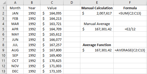
If I wanted to calculate the average for the year 1992, I could total the values relating to those years and then divide it by 12. The total comes to $2,007,617 and after dividing it by 12, I get an average of $167,301.42. But I can skip the step that involves dividing the data by using the Average function. Here’s a look at the difference:

Average calculations.

However, there’s a way we can simplify this even further. In this example, we still have to manually select the range that we want to average, and that’s not going to be optimal if you want to pull the average for every year. It’s also easy to make a mistake.

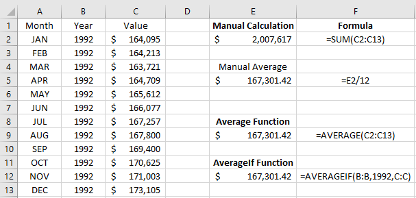
What we can use is the AVERAGEIF function in Excel. That function allows you to add criteria to your average. Here, we’ll use the year, 1992, as the criteria. And by doing so, we don’t have to worry about selecting the right cells since we can just select the entire column:

Averageif calculation.

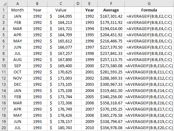
You’ll notice the year is hardcoded, which isn’t ideal. Here’s how we can fix that while also making it easy to pull the average by year:

Averageif calculation by year.

This is a great way to average by year, but it’s still not a moving average. Let’s do that next.

How to make the average move with your data

Companies often track sales numbers for the last 12 months, also referred to as the trailing twelve months (TTM). It’s actually easier to do than averaging by year since there’s no criteria — you’re simply averaging the last 12 months. The one limitation here is that you have to have 12 months of data before you can start. Here’s how that would look in our example:

Simple moving average calculation.

It’s as easy as just selecting the previous 12 cells in the range, averaging them, and copying the formula down. However, you don’t have to select the data range, even if it is just a one-time thing. If you include the OFFSET function, you can make your formula a lot more adaptable and flexible. It allows you to move your data set, and you can also determine how many values you want to include in your average.

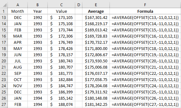
Here’s how a TTM calculation could look like using OFFSET:

Moving average calculation using offset.

This is a more complicated formula so let’s breakdown what’s happening here. The OFFSET function has multiple arguments, here’s a list of them:

  • Reference
  • Rows
  • Columns
  • Height
  • Width

The reference is just your starting point. In the first formula, I used cell C13 as that was the current value. It wouldn’t make sense to use data from a different row and I also want to make sure it’s in the value column since that’s where I want my data to come from.

Next, is the rows argument. I put -11 in this case because I want to start 11 rows higher than where the reference cell (C13) is. Moving 11 cells up would put me at C2, which is the first data point. The columns argument is left at 0 because I want to remain in the same column.

The height argument is key here because I want to ensure my data set contains 12 values in it. Without this argument, I would simply get the value from cell C2, $164,095. You can ignore the width argument or set it to 1, since you don’t need to include other columns.

If your data is organized in columns rather than rows, all you’ll need to do here is to switch around the arguments (e.g. rows would be in columns, height argument would go into width, etc.)

The last part of the formula is enclosing it within the average function so that it calculates the average.

Changing the number of periods you want to average

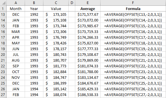
The big advantage of using the OFFSET function is now it’s a lot easier to manipulate your data and change how many values you want to include in your calculation. Suppose that instead of the last 12 months, we wanted to do a three-month average. All that would include is tweaking the OFFSET function so that it goes two rows back and includes three values. Here’s how that would look:

Moving average calculation using offset.

The key takeaway here is that the number of rows or columns that you want to go back will be one less than the number of rows or columns you want to include. The only exception would be if you don’t want to include the current month’s data. For instance, if in the December moving average you didn’t want to include December’s data and wanted to go from September-November, then you would offset three rows rather than two.

How a moving average can help smooth trends

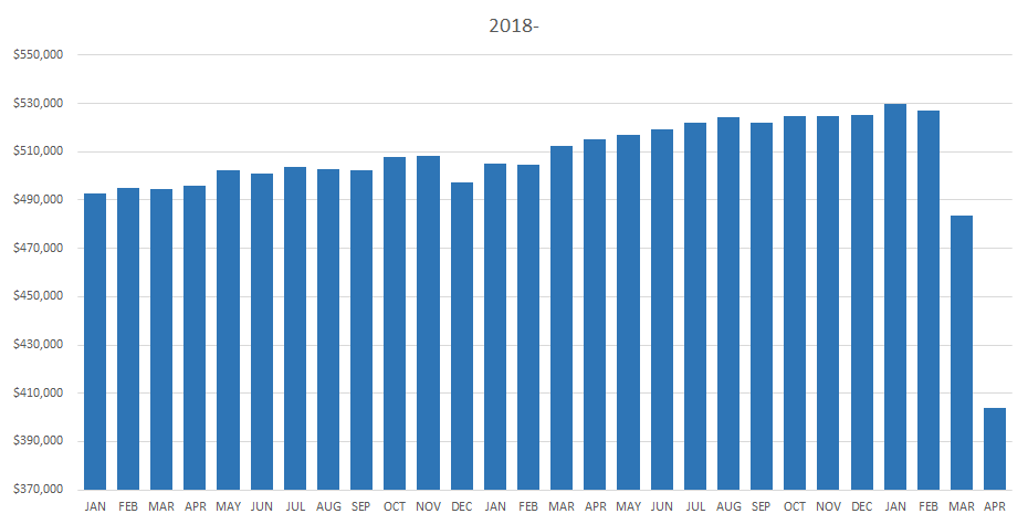
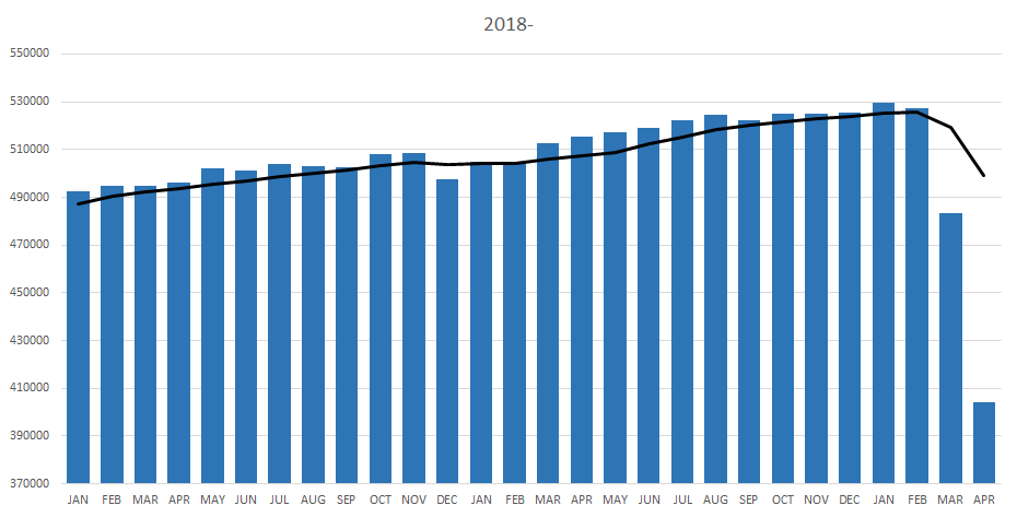
If we were to look at the data since 2018, here’s how it would look in a chart:

Monthly sales data on a chart.

It’s fairly stable and there aren’t any big jumps from one month to the next. Here’s how it would look with a three-month moving average:

Monthly sales data on a chart along with a six-month moving average.

Using the moving average, we can see what the longer-term trend is. You’ll notice that in the drop off that happened in March and April, the average goes on a much smaller decline because it’s still including earlier months in the calculation. And if we use a six-month average, then there’s even less of a dip in the trend:

Monthly sales data on a chart along with a six-month moving average.

Which period you use for a moving average will ultimately depend on how much smoothing you want. A short timeframe will be more volatile than a longer one, but a longer one may take too long to capture any changes.

That’s a quick overview of how to calculate moving averages in Excel. As you can see, you can just quickly grab an average or you can build a versatile formula using the OFFSET function which can make your calculations easier to change in the future.


If you liked this post on how to do a moving average in Excel, please give this site a like on Facebook and also be sure to check out some of the many templates that we have available for download. You can also follow us on Twitter and YouTube.

Calculating and Tracking Streaks with a Custom Function

With the stocks markets tanking earlier this month, I thought it’d be interesting to track their historical performance and put into perspective just how badly things have been going lately. For those that don’t know, one of my side jobs is writing articles for the Motley Fool Canada and so naturally this example attracted my interest.

However, there’s not an easy way to calculate this in Excel, and so I decided to go the route of a custom function.

What I’m going to be looking to accomplish is a way to to track how many consecutive trading days that a stock has been up or down, and then also calculate the cumulative value of those gains and losses.

If you’d like to follow along with my example, you can download the file I used here (you’ll have to save the file, open it in Excel and enable content, otherwise you’ll see NAME? errors)

Setting Up the Variables


I want the calculation to start from the bottom (the current cell) and work its way back up, since the latest results will be at the bottom. To do this I create a ‘bottom’ variable that looks like this:

————————————————————————————————————–

bottom = selection.Count + selection.Row – 1

————————————————————————————————————–

I want the user to be able to select what range they want the calculation to apply to, rather than selecting everything.

I also setup a variable for the column, which I named as offsetnum:

————————————————————————————————————–

offsetnum = selection.Column

————————————————————————————————————–

These two variables allow me to set my starting point for my calculation.

Determining if I’m Counting Negatives or Positives

The value of the starting cell will determine if I am going to be looking for positive numbers (gains) or negatives (losses), and so I setup an if statement to determine whether the first value is a gain or loss:

————————————————————————————————————–

If Cells(bottom, offsetnum) < 0 Then
    posneg = “negative”
Else
    posneg = “positive”
End If

————————————————————————————————————–

Start counting


The final step involves counting the values depending on whether I’m looking for positives or negatives:

————————————————————————————————————–

For counter = bottom To 1 Step -1

    If posneg = “negative” Then
 
            If Cells(counter, offsetnum) < 0 Then
                streak = streak – 1
            Else
                Exit For
            End If
         
      Else
   
            If Cells(counter, offsetnum) >= 0 Then
                streak = streak + 1
            Else
                Exit For
            End If
         
        End If
     

Next counter

————————————————————————————————————–

My complete function looks as follows:

————————————————————————————————————–

Function streak(selection As Range)

Application.Volatile
Application.Calculate

Dim bottom, offsetnum As Integer
Dim posneg As String

bottom = selection.Count + selection.Row – 1
offsetnum = selection.Column

‘Determine first value
If Cells(bottom, offsetnum) < 0 Then
    posneg = “negative”
Else
    posneg = “positive”
End If

For counter = bottom To 1 Step -1

    If posneg = “negative” Then
 
            If Cells(counter, offsetnum) < 0 Then
                streak = streak – 1
            Else
                Exit For
            End If
         
      Else
   
            If Cells(counter, offsetnum) >= 0 Then
                streak = streak + 1
            Else
                Exit For
            End If
         
        End If
     

Next counter

End Function

————————————————————————————————————–

Calculating consecutive points gains and losses


Now that I have a function to tell me the current winning or losing streak, I can calculate the cumulative gains and losses.
To do this, I am going to sum as far as the streak goes. And so far starters, I’m going to start with the SUM function. I am also going to use the OFFSET function because I need to determine how many rows up I need to add. The OFFSET will start from the current position and determine how far back I need to go to add up the totals in the current streak.

However, because some streaks are negative, I’ll need to also use the ABS function to just grab the number, regardless of if it is positive or negative. My formula looks like this so far:

=SUM(OFFSET(H2,1-ABS(I2), 0

Column H is where my gain or loss value is, while column I is the streak value. Since I want to sum the cumulative gains, I need to reference column H as my starting point.

I added the 1- before the ABS function because that will ensure the number is a negative, meaning that my formula will calculate upward, rather than downward if the number were positive. I also have to decrease the number of cells to offset because I don’t want to include the current cell, otherwise the formula will go too far.

Since I’m not offsetting any columns I set the next argument to 0.

The last argument I need to enter is the height of the offset function, otherwise the formula will just offset by the number specified in the second argument and pull that value, rather than pulling all the values that fall within the range.

This actually involves just copying the same argument again, but this time for the height. My completed formula looks as follows:

=SUM(OFFSET(H2,1-ABS(I2),0,ABS(I2)))

Note

Sometimes with custom functions you might notice that your calculations hang or stop computing correctly. What that means is you just need to recalculate using either F9 or you can edit in the cell and click enter, which will normally trigger a recalculation as well.

Alternatively what you could do is after running the formulas for the dataset, copy them over as values to ensure that they don’t change, since in this case you likely wouldn’t need to recalculate the streak value again.