How to Do a Moving Average in Excel

If you’re doing any type of data analysis, a moving average can be useful in smoothing trends and normalizing data. Below, I’ll show you how you can easily create a moving average in Excel. The data will again be based on the retail and food services sales data that I used in my post covering how to transpose data.

With the data now converted from the summary table, it’s in the right format for analyzing and averaging the data.

Calculating an average

To calculate an average in Excel, all you need to do is use the AVERAGE function. Simply select the range that you want to average, and the function will take care of the calculation for you. Here’s an excerpt from the data set:

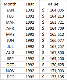
If I wanted to calculate the average for the year 1992, I could total the values relating to those years and then divide it by 12. The total comes to $2,007,617 and after dividing it by 12, I get an average of $167,301.42. But I can skip the step that involves dividing the data by using the Average function. Here’s a look at the difference:

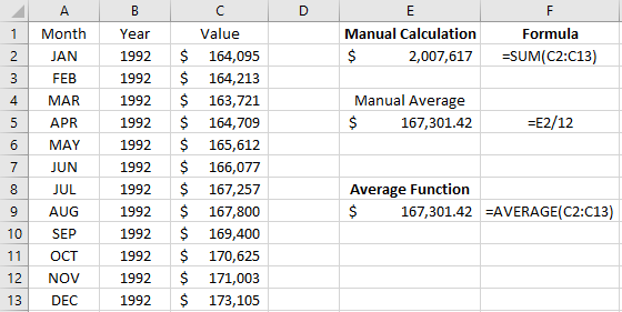
However, there’s a way we can simplify this even further. In this example, we still have to manually select the range that we want to average, and that’s not going to be optimal if you want to pull the average for every year. It’s also easy to make a mistake.

What we can use is the AVERAGEIF function in Excel. That function allows you to add criteria to your average. Here, we’ll use the year, 1992, as the criteria. And by doing so, we don’t have to worry about selecting the right cells since we can just select the entire column:

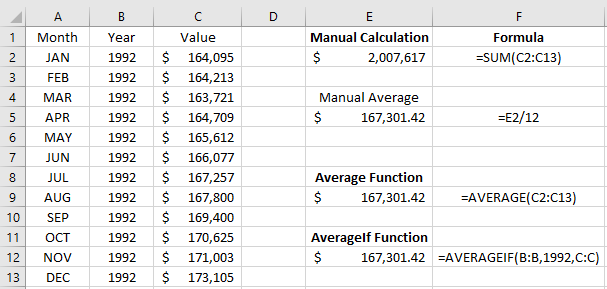
You’ll notice the year is hardcoded, which isn’t ideal. Here’s how we can fix that while also making it easy to pull the average by year:

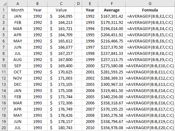
This is a great way to average by year, but it’s still not a moving average. Let’s do that next.

How to make the average move with your data

Companies often track sales numbers for the last 12 months, also referred to as the trailing twelve months (TTM). It’s actually easier to do than averaging by year since there’s no criteria — you’re simply averaging the last 12 months. The one limitation here is that you have to have 12 months of data before you can start. Here’s how that would look in our example:

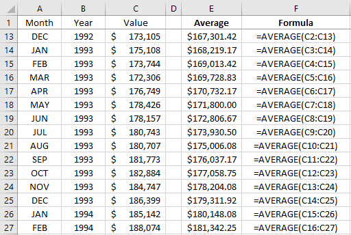
It’s as easy as just selecting the previous 12 cells in the range, averaging them, and copying the formula down. However, you don’t have to select the data range, even if it is just a one-time thing. If you include the OFFSET function, you can make your formula a lot more adaptable and flexible. It allows you to move your data set, and you can also determine how many values you want to include in your average.

Here’s how a TTM calculation could look like using OFFSET:

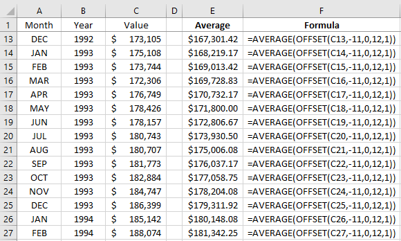
This is a more complicated formula so let’s breakdown what’s happening here. The OFFSET function has multiple arguments, here’s a list of them:

• Reference
• Rows
• Columns
• Height
• Width

The reference is just your starting point. In the first formula, I used cell C13 as that was the current value. It wouldn’t make sense to use data from a different row and I also want to make sure it’s in the value column since that’s where I want my data to come from.

Next, is the rows argument. I put -11 in this case because I want to start 11 rows higher than where the reference cell (C13) is. Moving 11 cells up would put me at C2, which is the first data point. The columns argument is left at 0 because I want to remain in the same column.

The height argument is key here because I want to ensure my data set contains 12 values in it. Without this argument, I would simply get the value from cell C2, $164,095. You can ignore the width argument or set it to 1, since you don’t need to include other columns.

If your data is organized in columns rather than rows, all you’ll need to do here is to switch around the arguments (e.g. rows would be in columns, height argument would go into width, etc.)

The last part of the formula is enclosing it within the average function so that it calculates the average.

Changing the number of periods you want to average

The big advantage of using the OFFSET function is now it’s a lot easier to manipulate your data and change how many values you want to include in your calculation. Suppose that instead of the last 12 months, we wanted to do a three-month average. All that would include is tweaking the OFFSET function so that it goes two rows back and includes three values. Here’s how that would look:

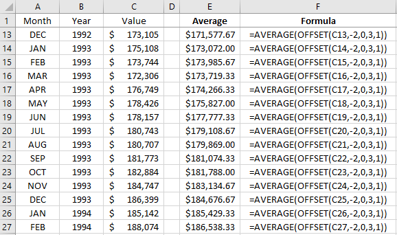
The key takeaway here is that the number of rows or columns that you want to go back will be one less than the number of rows or columns you want to include. The only exception would be if you don’t want to include the current month’s data. For instance, if in the December moving average you didn’t want to include December’s data and wanted to go from September-November, then you would offset three rows rather than two.

How a moving average can help smooth trends

If we were to look at the data since 2018, here’s how it would look in a chart:

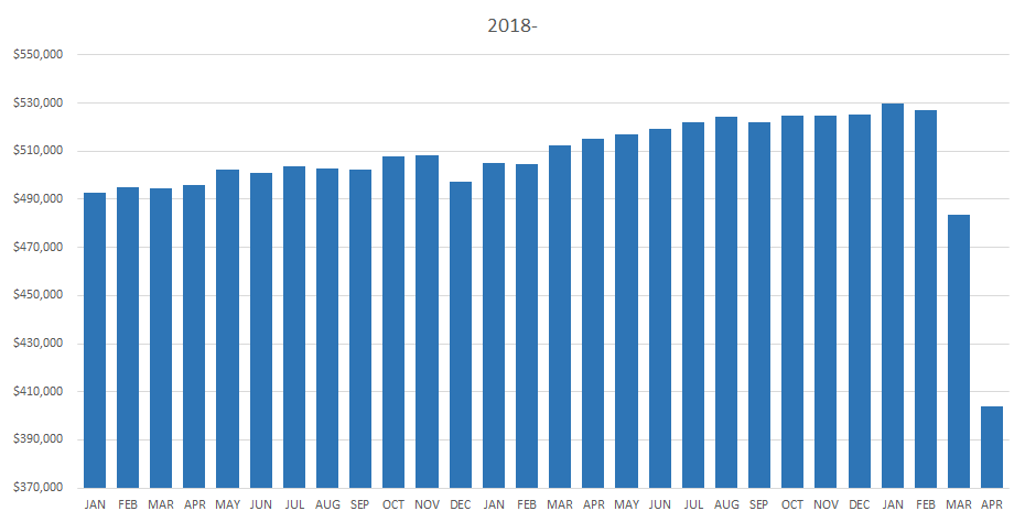
It’s fairly stable and there aren’t any big jumps from one month to the next. Here’s how it would look with a three-month moving average:

Using the moving average, we can see what the longer-term trend is. You’ll notice that in the drop off that happened in March and April, the average goes on a much smaller decline because it’s still including earlier months in the calculation. And if we use a six-month average, then there’s even less of a dip in the trend:

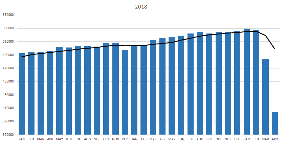
Which period you use for a moving average will ultimately depend on how much smoothing you want. A short timeframe will be more volatile than a longer one, but a longer one may take too long to capture any changes.

That’s a quick overview of how to calculate moving averages in Excel. As you can see, you can just quickly grab an average or you can build a versatile formula using the OFFSET function which can make your calculations easier to change in the future.

If you liked this post on how to do a moving average in Excel, please give this site a like on Facebook and also be sure to check out some of the many templates that we have available for download. You can also follow us on Twitter and YouTube.