Excel’s new functions help make it even easier to analyze and extract data efficiently and effectively. One example is extracting a list of unique values from a list. What you can also do is sort that list. Plus, you can then put all those values into a single cell, with each value separated by a comma. Data in the form of a comma-separated value (CSV) can make it easy to compile data into one place, without taking on too much space. In this article, I’ll show you how we can combine all this Excel functionality into one supercharged Excel formula that can do everything I’ve mentioned thus far. Let’s get started.
How to create a list of unique values for a specific criteria
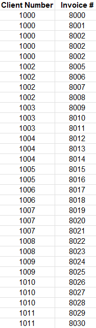
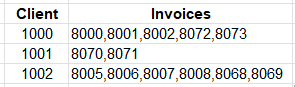
For starters, let’s get a list of unique values that meet a certain criteria. While pulling unique values isn’t terribly difficult in excel and there many ways to pull unique values, I’m going to show you how we can extract unique values that meet a given criteria. Here’s the data set I’ll be working with for this example:
It’s a straightforward list that includes a client number (column A) along with invoices (column B). But if I want to include just a list of the unique values relating to client 1000, the UNIQUE function on its own won’t help me with that. I need to apply a criteria first. To do this, I’ll first use the FILTER function. Using that function, here’s how I can grab all the values relating to client 1000:
=FILTER(B:B,A:A=1000)
The first argument in the formula is where I want to extract values from. The second argument pertains to my criteria, which is based on the values in column A. With this formula, this is my result:
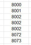
I get a list of values. But the problem is I have repeating values — invoice #8002 shows up multiple times. But I can put that formula to generate that list within the UNIQUE function:
=UNIQUE(FILTER(B:B,A:A=1000))
Now I have a condensed list which only includes unique values:
If your data isn’t sorted, you can also put this within the SORT function:
=SORT(UNIQUE(FILTER(B:B,A:A=1000)))
Now you have a formula that filters out data, grabs the unique values, and sorts them. It’s a busy formula. But it’s about to do even more.
Putting the list into a CSV format
As of now, the data is in a list. That’s not a convenient format because the danger is that you may have clients which have only a few invoices, perhaps none at all. Others, meanwhile, might have a dozen invoices. If you are creating arrays, they will inevitably vary in size, and the you’re left with a spreadsheet that doesn’t have much consistency to it.
To get around that, you can put your data in a CSV format. By doing so, you can ensure all of your data is contained within just a single cell.
Here’s the step-by-step process as to how you can put your data into a CSV format:
1. Use the TEXTJOIN function and use a “,” as you first argument. The first argument of this function tells you how you want to separate your data. By indicating a comma, you’re already setting up the result to be in a CSV format.
2. Set the next argument to TRUE. The second argument is whether you want to ignore empty values. You’ll likely want to ignore them, otherwise, you will have blank spaces between your commas.
3. Include your list of values. This is the data that you want to convert into a CSV.
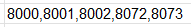
Here is what the complete formula looks like, with step 3 relating to the formula we created at the end of the previous section:
The list of unique invoice numbers is now within just a single cell. And each invoice is separated by a comma.
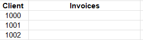
But let’s make this formula more dynamic. It should be able to generate a list based on each client, in the following table:
With the client values in column D, starting with cell D3, this is how I can adjust the formula so that it is not referencing a hardcoded invoice number:
Using that formula, the table will now populate the list of unique invoices for each client:
If you like this post on How to Extract and List Unique Values in Excel Into CSV Format, please give this site a like on Facebook and also be sure to check out some of the many templates that we have available for download. You can also follow me on Twitter and YouTube. Also, please consider buying me a coffee if you find my website helpful and would like to support it.
Replacing values can be an important part of cleaning up your data and preparing it for data analysis. Below, I’ll outline the steps to take to replace a value in Power Query. I’ll also show you how you can create a formula in Power Query to make it easy to replace multiple values at once.
Replacing a single value in Power Query
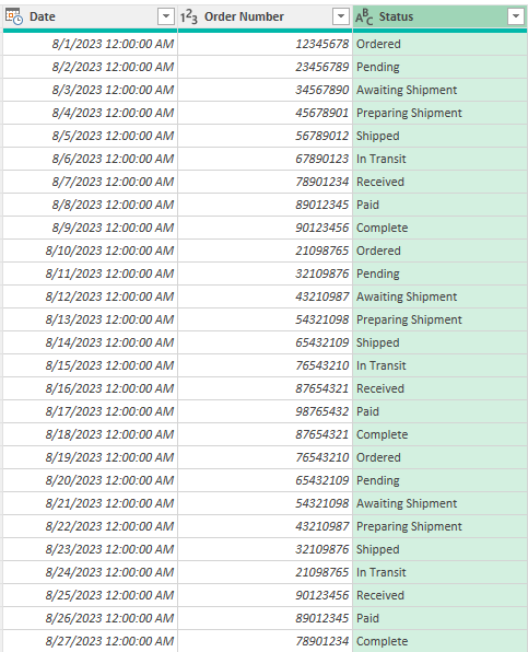
In the following data set, I have a list of orders. There are dates, order numbers, and statuses. Some of the statuses may be a bit similar so to reduce the number of them, it can make sense to replace values.
I am going to replace to the ‘Awaiting Authorization’ status to ‘Pending’.
Here are the steps needed to take to replace a value in Power Query:
1. Load your data into Power Query.
2. Right-Click on the column where you want to replace values and select Replace Values
3. Enter the value to find and what to replace it with, and then click OK.
Now, Power Query will replace the value for you:
This isn’t an ideal solution, however, because doing it this way would require you to repeat these steps over and over again. Instead, there’s another way to do this.
Replacing multiple values in Power Query at once
If you want to replace multiple values in a single step in Power Query, you can accomplish that through a formula. The Table.ReplaceValue function allows you to specify the values you want to replace. For instance, to replace just a single value, this would be the formula:
Where #”Changed Type” is the name of the preceding step. In this formula, any instance of ‘Awaiting Authorization’ is replaced with ‘Pending’.
If you want to replace multiple values, then you can use if statements to check for multiple conditions:
= Table.ReplaceValue(#"Changed Type",each [Status], each if [Status] = "Awaiting Authorization" then "Pending" else if [Status] = "Awaiting Shipment" then "Pending" else [Status], Replacer.ReplaceText,{"Status"})
The same function is used. However, by using the ‘each’ keyword, it will now cycle through the values in the [Status] field. It will do the original search for ‘Awaiting Authorization’ and replace it with ‘Pending’. There is also an else if statement which allows the formula to go even further and also replace ‘Awaiting Shipment’ with ‘Pending’. Finally, if there are no matches for either of those terms, then it will just leave the value that is already in the ‘Status’ field.
You can even add more else if statements to replace more values if necessary. By doing this, you can make the process even more efficient by swapping out even more values through a single step.
If you liked this post on How to Replace Multiple Values in Power Query, please give this site a like on Facebook and also be sure to check out some of the many templates that we have available for download. You can also follow me on Twitter and YouTube. Also, please consider buying me a coffee if you find my website helpful and would like to support it.
The TREND function in Excel is a powerful tool that allows users to perform linear regression analysis and make predictions based on existing data. This function is particularly valuable for professionals dealing with data analysis, financial modeling, and forecasting. In this article, I will go over how the function works, and provide step-by-step instructions on how to utilize it in your Excel worksheets.
Using the TREND function
To use the TREND function, follow the steps below:
1. Organize the data
Before you can use the function, you need to have your data organized so that it includes at least two columns. One needs to be for the independent variables, or the x-values, and another one for the dependent variables, or y-values. It is necessary for the data to be aligned correctly so that the information correctly relates to one another (i.e. you don’t want the wrong values lined up next to one another).
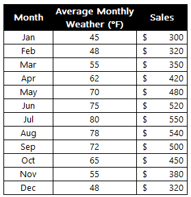
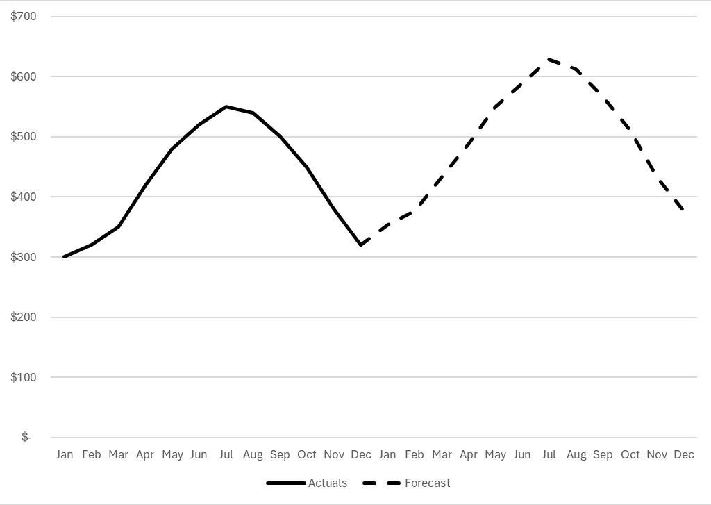
Below is sample data for a company which sells seasonal products. In warmer weather, revenue rises while in cooler temperatures, sales are lower.
2. Calculate the Trend Line
With the data populated, you can now enter it into the TREND function in Excel. This involves specifying the following arguments:
known_y’s
known_x’s
new_x’s
constant
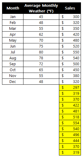
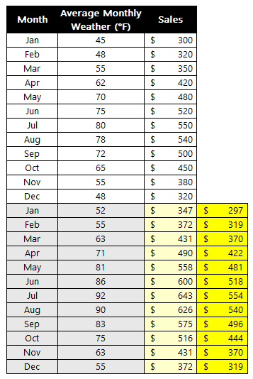
In the above example, the known_y’s are the sales, the known_x’s are the average monthly temperatures. If I don’t fill in any new_x’s or specify the constant, the function will still try and plot out the rest of the values:
The problem in this scenario is that it doesn’t take into account the temperature; it simply assumes a similar trend as before. The function is much more useful if I have forecasted monthly temperatures. That way, the trend calculation will take that into account. Suppose I fill in the data, telling Excel that I expect the temperatures to be much warmer over the next 12 months:
With the previous forecast off to the right, you can see that the TREND function has adjusted to reflect the newer information. Thus, the more data you plug into the function, the more reliable the forecast will be. Otherwise, it will simply assume the same patterns will repeat from before, which may not necessarily be the case.
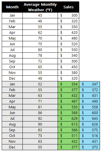
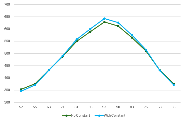
There is an additional argument in the function that you can also adjust, and that is the constant. If you set it to false it will be 0. If set to true, then the formula will calculate it. This is the b variable which is part of the y=mx+b equation. If you expect there to always be a minimum, a constant amount, then you may want this to be calculated. If, however, the data can fluctuate wildly, then you may want to set it to true so that there is no intercept. Here’s a comparison with the above data both when there is a constant and when there isn’t:
The forecast in green is where the argument is set to false (constant is set to zero) and blue is where it is true and a constant is calculated. From the chart below, you can see that there isn’t a big difference but the highs are higher and the lows are lower when there is a constant. This may, however, not always be the case as it will depend on your individual data set.
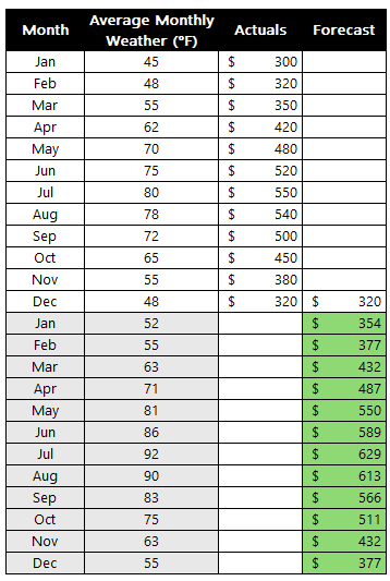
Create a chart to differentiate between actuals and forecast
One thing you may find helpful to do when creating a forecast is to put those amounts on a different column:
By doing this, you leave yourself space to add actuals later on and to compare them against your forecast. You can also create a chart with the forecast being a different series. In the below chart, I have used a dotted line to show the forecast while the actuals remain solid. For the first forecast amount, I set it to the same as the actual. This way, when I create the chart below, there are no gaps and it is merely a continuation of the line.
If you liked this post on How to Use the Trend Function in Excel, please give this site a like on Facebook and also be sure to check out some of the many templates that we have available for download. You can also follow me on Twitter and YouTube. Also, please consider buying me a coffee if you find my website helpful and would like to support it.
Excel’s Power Query is a powerful data transformation and analysis tool that allows users to retrieve, clean, and shape data from various sources. While Power Query provides an extensive set of built-in functions, there may be scenarios where you need to perform custom operations on your data. This is where custom functions in Power Query come into play. In this article, I will go over how to create a custom function in Power Query that you can invoke and re-use.
Steps to creating a custom function in Power Query
Creating custom functions in Power Query involves using the M language, which is the scripting language underlying Power Query. It can be complicated to create but I’ll show you two ways you can create a function. The first method is directly through coding, the other is after converting a query into a function.
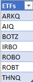
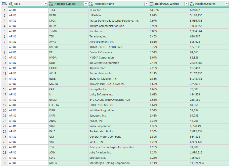
In this example, I’m going to pull all the stocks that are contained from a list of exchange-traded funds (ETFs). I’ve created the following table for this purpose, called tblETF:
Creating a custom function from scratch
If you’re creating a function in Power Query directly from code, here’s how to do that:
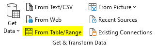
1. Go to load the data into Power Query by selecting a cell in your table, then click on the Data tab and click From Table/Range.
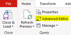
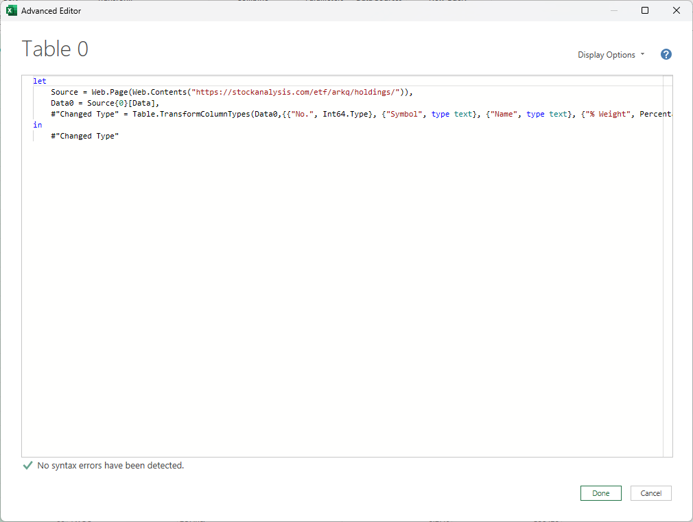
2. That will open up Power Query. Once there, on the Home Tab, click on the Advanced Editor button:
3. Create a name for the function using the let variable. In this example, I’m going to call it getholdings and it will pull all the holdings from the etf field. The opening line of the code is as follows:
let getholdings = (etf) =>
4. Next, list the commands that the function should execute. I’m going to pull the data from the stockanalysis.com page relating to the etf. This requires using the Web.Contents function and modifying the URL so that it includes the etf symbol:
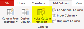
5. Now that the function is created, go into the query for the list of ETFs. Create an additional column from the Add Column tab, and select the button to Invoke Custom Function.
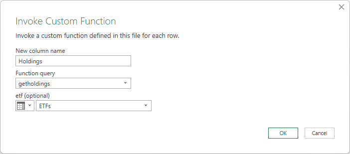
6. Set a column name for the new column. Then, specify the function query to reference. And you’ll also need to specify where the ETF value is coming from, which involves selecting the column:
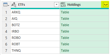
7. Next, you’ll expand the table that has been created within the column. This is done by pressing on the icon that shows arrows going in opposite directions. Then, select all the available columns.
You should end up with something that looks like this:
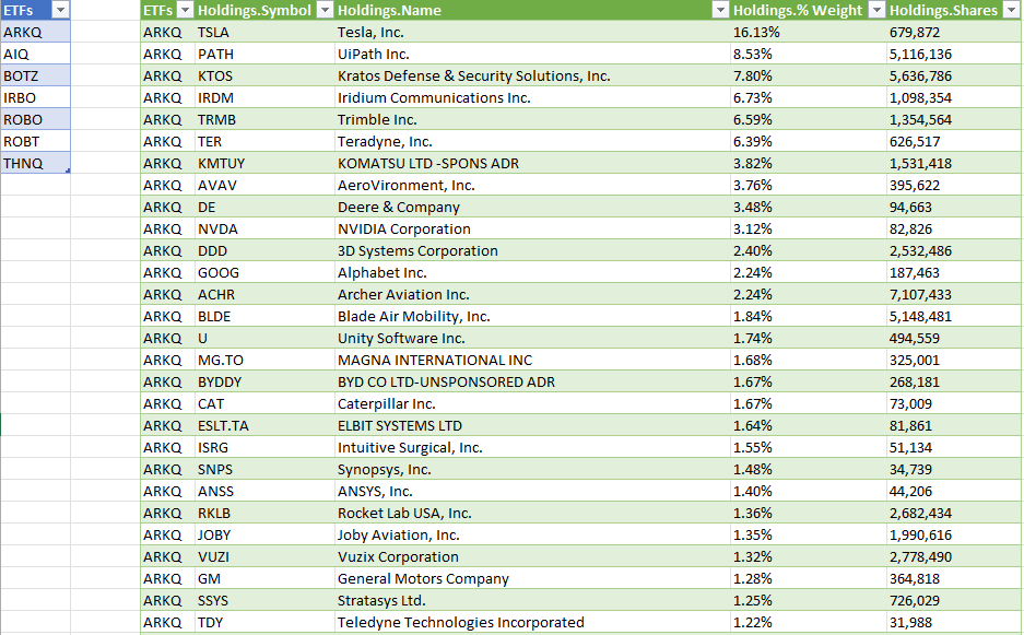
You can now click Close & Load and this data will load in your Excel spreadsheet. Now you can add to your ETF list and refresh the data, and the table of all the holdings will populate.
Converting a query into a function
If you’re not comfortable coding with Power Query, you can first create the steps, and then convert the query to a function.
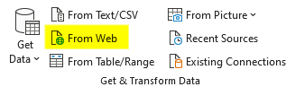
First, it’s necessary to create the query. In the previous example, I loaded the URL from a dynamic web page. To do that, I’ll start with selecting the From Web button on the Get & Transform Data section:
Next, populate the entire link, without the ETF variable — this will be added later:
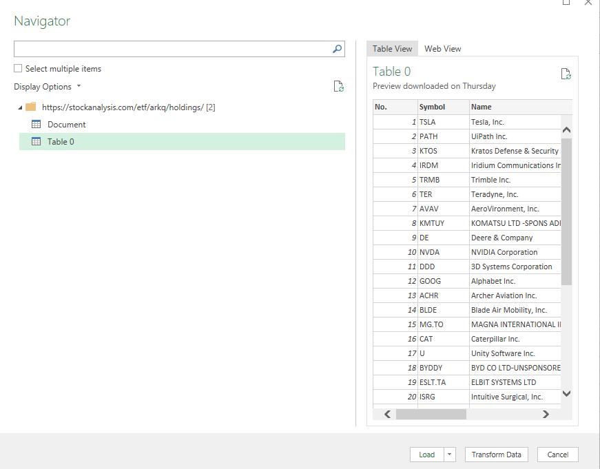
Then, select the table that contains the data and click the LoadTo button and select connection only:
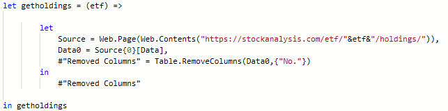
Then, right-click on the query to edit it so that you’re back in Power Query. From there, click on the Advanced Editor and you should see this:
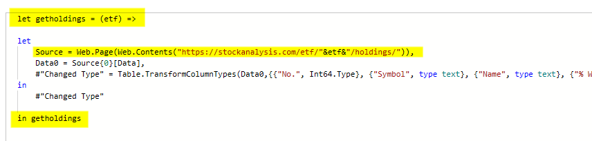
This is similar to the code in the first approach. To convert this into a function, we need to add another let variable and specify the function name, and any variables that will be used in the function. For the first line, I’ll add the following
let getholdings = (etf) =>
and for the URL, I’ll put the etf variable into there:
Here’s the updated code, with the changes highlighted in yellow:
Now I’ve converted my query into a function that can be invoked.
If you liked this post on How to Create a Custom Function in Power Query, please give this site a like on Facebook and also be sure to check out some of the many templates that we have available for download. You can also follow me on Twitter and YouTube. Also, please consider buying me a coffee if you find my website helpful and would like to support it.
Do you have multiple lists in Excel or Google Sheets that you want to combine together? With new functions such as VSTACK and HSTACK, you can do just that. In this post, I’ll show you how you can also filter out duplicates and apply sorting so that your data is organized after consolidating all of your lists.
Combining multiple stock lists into a large one
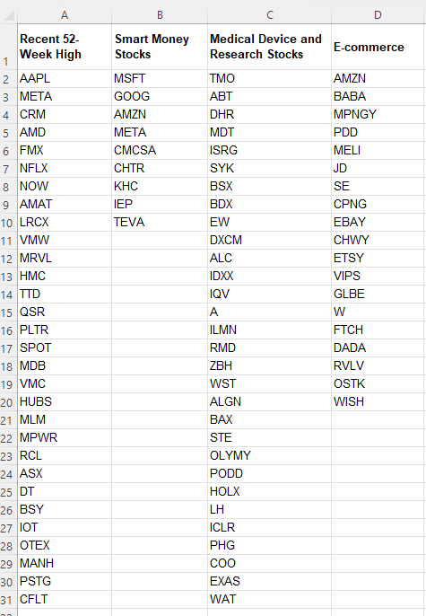
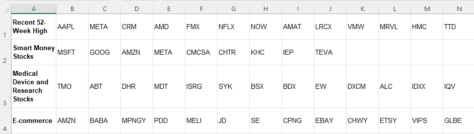
In this example, I’ll use various stock lists that I want to combine into one large list. On Yahoo Finance, you can find an assortment of different lists to help filter stocks. Below, I’ve pulled the lists of stocks that recently hit new 52-week highs, smart money stocks, medical device and research stocks, and e-commerce stocks:
The advantage of keeping the lists separate is that you can more easily update them. And by using VSTACK, you can combine these lists into a larger one so there’s no worry about having to consolidate them later on.
Based on the lists above, this is the formula that I use to combine them all together, using VSTACK:
=VSTACK(A2:A31,B2:B10,C2:C31,D2:D20)
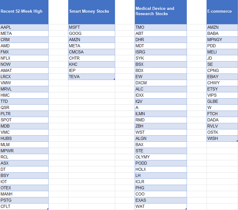
Since I don’t want to include the headers, I start from row 2. You’ll notice that I’ve hardcoded the ranges here. One way to make this more dynamic would be to use a COUNTIF or COUNTA function for the individual lists, and then use the INDIRECT function to limit the scope of the list. Another option involves converting the lists into tables. That way, you only have to list the table column and you don’t have to worry about the ranges. The one caveat here is that if you have lists that have different lengths, you’ll want to make each list its own table. Otherwise, Excel will automatically fill in the gaps with blank values:
While the data looks correct, if I were to use the VSTACK formula for these different table columns, I would get a consolidated list that involves many zero values. To keep it cleaner, it’s easier to just separate them into their own tables, and then reference them afterwards.
To reference these columns, my formula becomes much simpler:
=VSTACK(Table1[Recent 52-Week High],Table2[Smart Money Stocks],Table3[Medical Device and Research Stocks],Table4[E-commerce])
The advantage of doing it this way is that now I don’t have to worry about hardcoding the ranges, and thus, it’s easier to update.
Whichever method you prefer, the end result should look like a consolidated list:
Removing duplicates and sorting the list
In some of these lists, there is some overlap. AMZN and META are two stocks that show up twice. This means that my consolidated list will include those values multiple times. To get around this, I can embed the formula within the UNIQUE function:
=UNIQUE(VSTACK(A2:A31,B2:B10,C2:C31,D2:D20))
If you also want to sort your list, then you can add the SORT function as well:
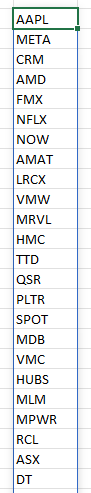
If you have the same lists but instead have them going horizontally, then you can use the HSTACK function. It works the same way as the VSTACK but as the H suggests, it will require horizontal arrays. Here are the same list of stocks as in the first example, this time transposed so that they go horizontally:
In this case, the formula for HSTACK would be as follows:
=HSTACK(B1:AE1,B2:J2,B3:AE3,B4:T4)
You can apply the same steps as for the VSTACK to eliminate duplicates and to sort the results.
These formulas work the same in Google Sheets as in Excel
Whether you’re working in Google Sheets or Excel, these formulas will be the same. The VSTACK, HSTACK, SORT, and UNIQUE functions are all available on the latest version of Excel and on Google Sheets. There is no need to change any of the formulas besides just adjusting for any difference in ranges. The formulas themselves work in the same ways, making it easy to transfer data between Google Sheets and Excel and to replicate these formulas wherever makes sense for you.
If you liked this post on How to Use VSTACK and HSTACK in Excel and Google Sheets to Consolidate Lists, please give this site a like on Facebook and also be sure to check out some of the many templates that we have available for download. You can also follow me on Twitter and YouTube. Also, please consider buying me a coffee if you find my website helpful and would like to support it.
Excel has many different functions that can help you parse out text from cells. This includes the LEN, MID, LEFT, and RIGHT functions. By utilizing these and other functions, you can get just the values you want. And by determining the number of blank spaces within a cell, you can also determine the number of words that a cell contains. There are multiple ways you can count cells in Excel, I’ll start with using the easier, and newer TEXTSPLIT function.
Method 1: Counting words using the TEXTSPLIT function
The TEXTSPLIT function is available for users who have Microsoft 365 and so if you do not see that function available as you type it in, you’ll need to move to the second approach. Using the TEXTSPLIT function, you can turn a single text value in a cell into multiple cells or columns. And you can specify how you want to split a cell; which delimiter you want to use.
In the example of counting words, the delimiter you would use is a blank space, as specified with ” ” in the delimiter argument. Here’s a list of article titles that I am going to use for this example:
The article titles are in column A. The formula to split the text every time there is a blank space would be as follows, assuming the first value is in cell A2:
=TEXTSPLIT(A2,” “)
This formula, however, would simply put all the words in different columns. Thus, it is incomplete when your goal is to count the number of words. To fix this, the formula needs to be embedded within the COUNTA function. How COUNTA works is that it simply counts the number of nonblank values.
=COUNTA(TEXTSPLIT(A2,” “))
Copying this formula down, these are the resulting values and the number of words found in each cell:
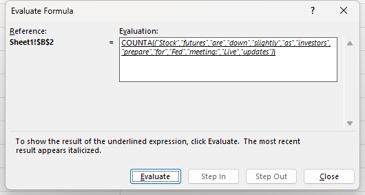
Here’s a closer look at how the formula in B2 works, using the Evaluate Formula feature in Excel:
The TEXTSPLIT function is breaking out each word as its own separate value. And the COUNTA function is then counting each one of those values. When combined, these functions allow you to count the number of words in a cell.
If you’re using Google Sheets, you can use the exact same formula as shown above, with the only difference being that instead of TEXTSPLIT, you’ll use the SPLIT function. It works in the exact same way.
Method 2: Using the LEN and SUBSTITUTE functions to count words
If you are on an older version of Excel where TEXTSPLIT isn’t available, there’s still a way that you can count the number of words within a cell. It will be a slightly more complex formula that will use the LEN and SUBSTITUTE functions.
The first part of the formula will involve counting the number of characters in a cell, which is what the LEN function does. This is accomplished through the LEN(A2) formula — assuming that A2 is where the article name is.
Next, you’ll need to use the SUBSTITUTE function to replace the blank values ” ” with an empty string that just contains two quotes: “”. To do that, the formula for that portion would be: SUBSTITUTE(A2,” “,””). This formula will need to be enclosed within a LEN function. What this accomplishes is it counts the number of characters in the cell after you’ve replaced all the blank values. If you take the total cell length and subtract this second piece, you’ll be left with the number of blank values in the text.
=LEN(A2)-LEN(SUBSTITUTE(A2,” “,””)
However, this isn’t entirely correct as you will be off by 1 word. This is because since the formula is counting the number of blanks, it won’t include the first word, which doesn’t come with a space before it. That also means if you only have one word, you’ll have a value of 0 instead of 1. To fix this, you’ll simply need to add a +1 to the end of your formula.
=LEN(A2)-LEN(SUBSTITUTE(A2,” “,””)+1
This would mean, however, that even blank cells would return a value of 1. And this would technically be the same problem when using the TEXTSPLIT function as well, since it doesn’t check for blanks, either. To correct this, you can simply add an IF function to check if the value is indeed blank. Here’s how the full formula looks:
This will return nothing if the cell is blank. If the cell isn’t blank, then it will go ahead and perform the rest of the calculation. As mentioned, this IF function can also be added to the start of the TEXTSPLIT function as well.
If you liked this post on How to Count Words in Excel, please give this site a like on Facebook and also be sure to check out some of the many templates that we have available for download. You can also follow me on Twitter and YouTube. Also, please consider buying me a coffee if you find my website helpful and would like to support it.
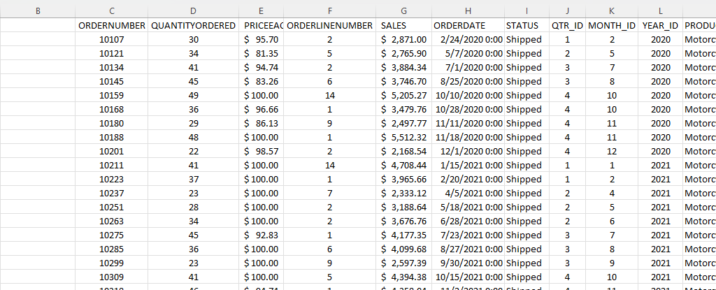
If you’re an accountant, you know that working with large amounts of data can be a daunting task. But with Excel, that work can get a whole lot easier and more efficient. Understanding Excel’s advanced features and functions can improve productivity, reduce errors, make your work more accurate, and most importantly — save you time. Below, I’ll go over some of the most important Excel functions that accountants should know, and provide examples of how to use them. For this example, I’ll use the following spreadsheet. Feel free to download it and follow along with the calculations.
1. SUM
The SUM function is a basic but essential function in Excel. It allows you to add up a range of values, which is helpful when calculating totals, such as revenue, expenses, and profits. Suppose you have a spreadsheet with sales data. In the above example, the total sales are in column G. If you wanted to sum up the entire column, the formula would be as follows: =SUM(G:G)
2. AVERAGE
The AVERAGE function calculates the average of a range of values. It is useful when analyzing data and preparing financial statements. In the above example, suppose you wanted to calculate what the average sale was. To do this, you can just use the AVERAGE function on column G, similar to the SUM function before. Here’s the formula: =AVERAGE(G:G)
3. IF
The IF function allows you to test a condition and return one value if the condition is true and another value if the condition is false. This can be useful because it can send your formulas to the next level. By knowing to use the IF function, you could also use SUMIF, AVERAGEIF, and many other functions that involve an if statement. In the above example, let’s say you only wanted to know if a value in cell M2 was part of the Motorcycles product line. The formula would be as follows: =IF(M2=”Motorcycles”,1,2). If it is part of Motorcycles, you would have a value of 1, otherwise, it would be 2.
4. SUMIF
By knowing the SUM and IF functions, you can combine them together with SUMIF, which is an incredibly popular function. It gives you a quick way to tally up the totals that meet a criteria. For example, let’s say you want all sales that relate to the Motorcycles category. The formula for that would be as follows: =SUMIF(M:M,”Motorcycles”,G:G). If the criteria is met in column M, then the formula will sum up the corresponding values in column G. There’s also the super-powered SUMIFS function, which allows you to combine multiple criteria.
5. EOMONTH
The EOMONTH function calculates the last day of the month for a specified number of months in the future or past. It is useful when working with data that is organized by date. For accountants, this can be useful when you’re calculating when something is due. Let’s say in this example, we need to calculate the date orders need to go out on, and that needs to be the end of the next month. Using the ORDERDATE field in column H, here’s how that calculation would look in the first cell, which would then be copied down for the rest: =EOMONTH(H2,1)
6. TODAY
The TODAY function is helpful for accountants in calculating deadlines and knowing how many days are remaining or past a certain date. Suppose that you wanted to know how many days have past since the ORDER DUE DATE that was calculated in the previous example. Rather than entering in a static date that every day you would need to change, you can just use the TODAY function. Here’s how a formula calculating the days since the deadline for the first cell would look like, assuming the due date is in column N: =TODAY()-N2. The next day you open up the workbook, the calculations will update to reflect the current date; there’s no need to make any changes. There are many more date calculations you can do in Excel.
7. FV
The FV function calculates the future value of an investment based on a fixed interest rate and a regular payment schedule. You can use it to calculate the future value of an investment or savings account. Let’s say that you wanted to save $10,000 per year and expect to earn a return of 5% per year on that investment. Using the FV calculation, you can do that with the following formula: =FV(0.05,5,-10000). If you don’t enter a negative for the payment amount, the formula will result in a negative value. You can also specify whether payments happen at the beginning of a period (1) or end (0 — this is the default) with the last argument in the function.
8. PV
The PV function lets you do the opposite and work backwards from a future value to the present. Knowing that the calculation in example 7 returns a value of $55,256.31, that can be used in the PV calculation to check our work: =PV(0.05,5,10000,-55256.31). The formula returns a value of 0, which is correct, as there was no starting value in the FV calculation.
9. PMT
The PMT function calculates the periodic payment required to pay off a loan with a fixed interest rate over a specified period. It is helpful when determining the monthly payments required to pay off a loan or mortgage. Let’s take the example of a mortgage payment where you need to pay down $500,000 over the period of 30 years, in monthly payments. At a 5% interest rate, here’s what the payment calculation would be: =PMT(0.05/12,12*30,-500000,0). Here again the ending value needs to be a negative to avoid a negative value in the result. And since the payments are monthly, the periods need to be multiplied by 12 and the interest rate is dividend by 12.
10. VLOOKUP
The VLOOKUP function allows you to search for a value in a table and return a corresponding value from another column in the same row. It’s one of the most common Excel functions because of how useful and easy to use it is. It is helpful when working with large data sets and performing data analysis. Let’s suppose in this example that you want to find the sales related to order number 10318. The formula for that calculation might look like this: =VLOOKUP(10318,C:G,5,FALSE). In a VLOOKUP function, you need to specify the column number you want to extract from, which is what the 5 represents. If you’re using Office 365, you can also use the newer, flashier XLOOKUP function. I put VLOOKUP on this list because it’ll work on older versions of Excel — XLOOKUP won’t.
11. INDEX
The INDEX function allows you to return a value from a data set by specifying the row and column number. It’s also helpful if you just want to return data from a single row or column. For example, the sales column is in column G. If I know the order number is on row 20 (which relates to order number 10318), this formula would do the same job as the VLOOKUP in the previous example: =INDEX(G:G,20,1).
12. MATCH
The MATCH function allows you to find the position of a value within a range of cells. Oftentimes, Excel users deploy a combination of INDEX and MATCH instead of VLOOKUP due to its limitation (e.g. VLOOKUP can’t extract values to the left of the lookup field). In the previous example, you had to specify the row belonging to the order number. But if you didn’t know it, you could use the MATCH function within the INDEX function. The MATCH function would look like this: =MATCH(10318,C:C,0). Placed within an INDEX function, it can replace the argument where in the previous example, we set a value of 20: =INDEX(G:G,MATCH(10318,C:C,0),1). By doing this, you have a more flexible version of the VLOOKUP function. You can also create dynamic formulas using INDEX and MATCH that use lookups for both the column and row.
13. COUNTIF
The COUNTIF function allows you to count the number of cells in a range that meet a specified condition. Let’s count the number of values in the data set that are Motorcycles. To do this, you would enter the following formula: =COUNTIF(M:M,”Motorcycles”).
14. COUNTA
The COUNTA function is similar to the previous function, except it only counts the number of non-empty cells. With no criteria, it is helpful to just the total number of values within a range. To calculate how many cells are in this data set, you can use the following formula: =COUNTA(C:C). If there are no gaps in data, then the result should be the same regardless of which column is used. And when combined with the UNIQUE function, you can have an easy way to count the number of unique values.
15. UNIQUE
The UNIQUE function returns a list of unique values within a range, and it’s a much easier method than the old-school way of extracting unique values. If you wanted to extract all the unique product lines in column M, you would enter the following formula: =UNIQUE(M:M). If, however, you just wanted to count the number of unique values, you could embed it within the COUNTA function as follows: =COUNTA(UNIQUE(M:M)). You can adjust your range if you don’t want to include the header.
This is just a sample of some of the useful Excel functions that accountants can utilize. If you are familiar with them, you’ll put yourself in a great position to improve the efficiency of your workflow and make your spreadsheets easier to use. Plus, you can confidently say that you are highly competent with Excel, which can make your resume more attractive and make you better suited for accounting jobs that require advanced Excel skills — and there are many of them that do!.
If you liked this post on 15 Excel Functions Accountants Should Know, please give this site a like on Facebook and also be sure to check out some of the many templates that we have available for download. You can also follow me on Twitter and YouTube. Also, please consider buying me a coffee if you find my website helpful and would like to support it.
Want to show your data in reverse order, and want to do so without having to sort it? Using just a formula, you can change the way your data looks. Instead of going from oldest to newest, you can display it from newest to oldest. And you don’t have to alter your existing data set to do it. In this post, I’ll show you can how can flip your data through just a single formula.
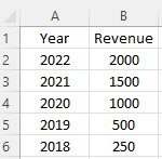
In the below example, I have data going in descending order by year.
If I wanted to change the order so that it’s in ascending order, I could use the sort button. But what if you needed to keep the data the way it is and I just wanted to put in different order, say for the sake of a chart or report. I can accomplish this using the functions INDEX, ROW, and COUNTA. Here’s how it works.
Creating the formula to flip data
The first function I’m going to use is the INDEX function. This is important because this function will include all the data that I need. Since my data is in the range A1:B6, I’ll start with a formula to get the years in column A and reverse them. The formula will start as follows
=INDEX(A$1:A$6
I’m freezing the row numbers because I want to ultimately copy this formula over to the revenue column, and flip those values as well. In the next part of my formula, I will need to grab a count of the values in my range. This can be achieved by using the COUNTA function:
=INDEX(A$1:A$6,COUNTA(A$1:A$6)
The above formula would grab the last value in the range. And while that’s technically what I want, the formula wouldn’t work if I were to copy it down. Thus, I need to add a 1 to it and I also need a way to also deduct 1 — for the first instance, anyway. To make it dynamic, I’m going to use the ROW function.
=INDEX(A$1:A$6,COUNTA(A$1:A$6)+1-ROW(A1))
How this works is that the formula will grab a count of the rows in the data set. Then the formula will add 1 but it will also deduct 1 using the ROW function. In this first formula, my value will be 6 — the same as the count of cells. However, if I drag it down, the formula for the next cell will be as follows:
=INDEX(A$1:A$6,COUNTA(A$1:A$6)+1-ROW(A2))
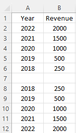
In the above formula, I’ll now be deducting 2 since the row value of A2 is 2. In this case, the row value I will be extracting is 5. The COUNTA function returns value of 6, then 1 is added, and the ROW function deducts 2. By dragging this formula down, it will now continue going backwards and so that the last value will be the first row. If I also copy this over to column B for revenue, I will now have both columns flipped and going in the opposite direction:
If you liked this post on How to Flip Your Data in Excel Without Sorting, please give this site a like on Facebook and also be sure to check out some of the many templates that we have available for download. You can also follow us on Twitter and YouTube.
Did you know that you can filter data by just using a single function in Excel? There’s no longer a need to use advanced filters or to manually select the data you want, you can just use the FILTER function, and it will give you an array of values that have met your criteria. By using the function, you can save time and make it easier to extract the data into another place on your spreadsheet.
Applying a single filter
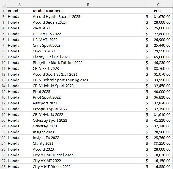
In the data set below, I have a list of makes and models of cars, and their prices.
Suppose you wanted to filter the data so that you only saw all the Ferraris on this list. You could use a normal filter in Excel to only see certain data. But by doing so, you will change the look of your data set. With the FILTER function, you can create a formula in another part of your spreadsheet and apply the filter you want to use.
Here’s what the formula could look like:
=FILTER(A:B,A:A=”Ferrari”)
In the above formula, I’m selecting both columns A and B (brand and model.number), but I’m only filtering column A where it equals the value of Ferrari. Now, in the area where I’ve entered my formula, I get an array back of all the Ferraris, with the values that were in both A and B.
You can apply more advanced filters than this.
Applying multiple filters
Suppose you wanted to also apply a filter so that you can see the Ferraris that are over $500,000. This part can be tricky because there’s only one argument field for what to include. The key here is to create multiple rules, and then multiply them by one another to determine if the result is true (i.e. both criteria are met).
The second criteria will be to look at column C and check if the value is more than $500,000:
C:C>=500000
To combine both of the rules, the criteria need to multiply against one another. If a criteria is met, the result is 1 (True). If it isn’t met, then it is 0 (False). So if both criteria are met, it would be multiplying 1 x 1. And if it’s a 1, then the value gets included. Here’s how the full formula looks like:
=FILTER(A:B,(A:A=”Ferrari”)*(C:C>=500000))
By deploying multiple criteria, the list of Ferraris becomes much smaller:
You could also expand this criteria even further. To add another criteria, simply add another condition to multiply against. That way, you can have even more specific criteria to apply.
At the same time, you can use OR criteria. And this can be accomplished by adding instead of multiplying criteria. If instead of multiplying I add my criteria, now my filter will look for either a Ferrari or a car that is priced at $500,000 or over:
This now covers a much broader list that includes non-Ferrari vehicles. By using multiplication and addition, you can create a variety of different rules. The key to remember is that if the end result will be a 1 (True), then it is included. If it will be a 0 (False), then it won’t be.
If you liked this post on How to Use the Filter Function in Excel, please give this site a like on Facebook and also be sure to check out some of the many templates that we have available for download. You can also follow us on Twitter and YouTube.
Doing a simple summation in Excel is as easy as clicking on the AutoSum button or just using the SUM function. But in some cases, you don’t want to be summing up everything within a range. In those situations, you may want to use the SUBTOTAL function instead. In this post, I’ll go over how that function works, and illustrate the differences between it and SUM function.
What’s the difference between SUM and SUBTOTAL in Excel?
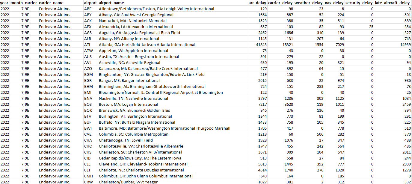
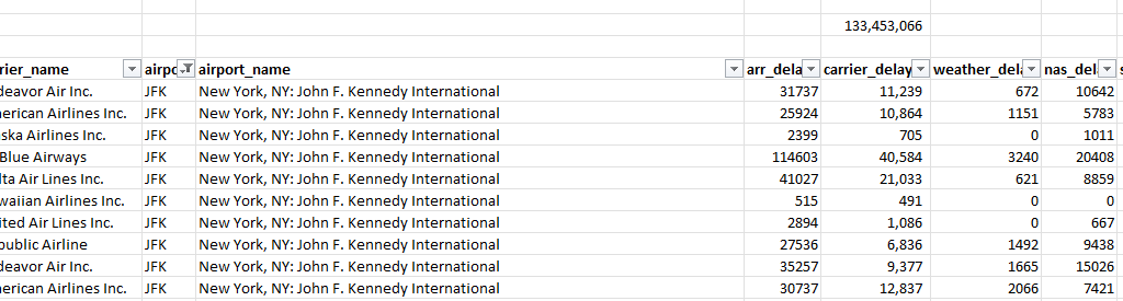
Suppose you have the following data set, which sows airport delays by carriers at different airports:
Using the SUM function on column header for carrier_delay, the total value comes out to 133,453,066. Even if you were to filter the data based on a single airport (in this example, JFK), the total value would remain the same:
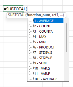
If you were to use the SUBTOTAL function, however, then it would only perform a calculation on the cells that are visible and filtered. If you’re using SUBTOTAL, you just need to specify the type of calculation you want to perform:
To do a summation, you just enter 9 for the first argument. As you can see, there are options to do COUNT, COUNTA, MAX, MIN, PRODUCT, AVERAGE, PRODUCT, standard deviation, and variance calculations. Once you specify the first argument, all you need to do after that is select the range as you would in a normal SUM formula. Here’s what the SUBTOTAL formula looks like in my spreadsheet, where I am adding up the values in column Q:
=SUBTOTAL(9,Q7:Q500000)
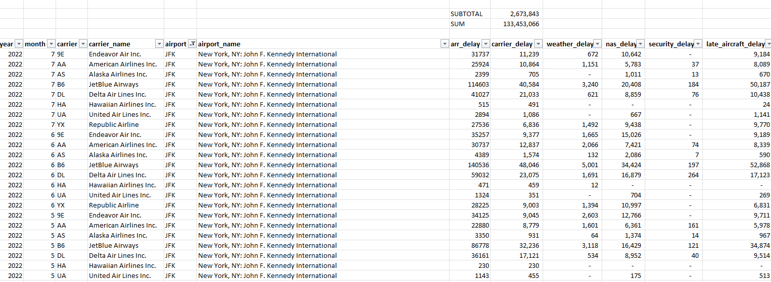
Now, there’s a difference between the SUM and SUBTOTAL formulas in their results:
If you were to change your filters and selections, the SUBTOTAL value would change while the SUM value would remain the same.
If you liked this post on When to Use Subtotals In Excel, please give this site a like on Facebook and also be sure to check out some of the many templates that we have available for download. You can also follow us on Twitter and YouTube.