How to Use Tags in Excel

Did you know that you can group numbers in Excel using tags? By just listing all the categories an item should belong to, you can make it easier to group them. In this post, I’ll show you how you can use tags in Excel to efficiently summarize different categories.

Creating tags

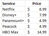
Suppose you wanted to list all the possible streaming services you might subscribe to. You might have a list that looks something like this:

This is fine if you want to compare them or even tally them all up. But what if you wanted to look at different scenarios, such as what if you select some of these services, but not all of them? This is where tags can be really helpful. Let’s say I want to create the following categories:

• Basic
• Kids
• Tier 1
• Tier 2
• Tier 3

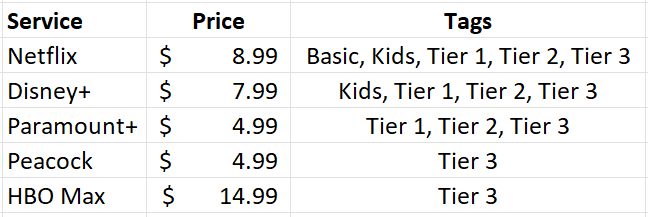
Each category will have a different mix of services. Here’s how I can use tags to make that happen. I’ll create another column next to the price where I specify all the categories a service will fall under:

In the above example, Netflix is included in every package but HBO Max is only included in Tier 3. Next, what I’m going to do is create columns for each one of these tags, such as follows:

Without using tags, you might be tempted to put a checkmark to determine which service belongs in which category. But that’s not necessary here. Instead, I’m going to use a function to determine whether to pull in the price or not.

Using a formula to determine if a tag is found

The key to making this work is the SEARCH function. This will look within the tag values to see if there is a match. If there is, then the price will be populated within the corresponding category. To check if the ‘basic’ keyword is found within the tags related to Netflix (assume this is cell C2), this is how that formula would look:

=SEARCH(“basic”,C2,1)

This will return a value of 1, indicating that the term is found at the very start of the string. If you use the function to look for the word ‘kids’ then it would return a value of 8 as that comes after ‘basic in my example.’ Of key importance here is that there is a number. If there isn’t a number and instead there is an error, that means that the tag wasn’t found. I will adjust the formula as follows to check if there is a number:

=ISNUMBER(SEARCH(“basic”,C2,1))

This will return a value of either TRUE or FALSE. But the formula needs to go further than just identifying if the tag was found. It needs to pull in the corresponding value. To do this, I’ll need an IF statement to extract the value from column B:

=IF(ISNUMBER(SEARCH(“basic”,C2,1)),B2,0)

By freezing the formulas and copying this across the other categories, this formula will now allow me to pull in the amounts correctly based on the tags:

But let’s say you don’t even want to do this, you just want to quickly group the totals without these extra columns. You can also do that with the help of tags.

Summarizing the totals by category

You don’t need to create a column for each group if you don’t want to. You summarize the total in just an array formula. Simply use the formula referenced earlier and include it within a SUM function, while referencing the entire range:

=SUM(IF(ISNUMBER(SEARCH(“basic”,C2:C6,1)),B2:B6,0))

This is the same logic as before, except this time the values will be totaled together. On older versions of Excel, you may need to use CTRL+SHIFT+ENTER after entering this formula for it to correctly compute as an array. But if you’re using a newer version, you don’t need to. If you copy the formula to the other categories, you’ll be able to sum the values by without the need for additional columns:

If you liked this post on Using Tags in Excel, please give this site a like on Facebook and also be sure to check out some of the many templates that we have available for download. You can also follow us on Twitter and YouTube.