Most people rely on online mortgage calculators in order to calculate and estimate their mortgage payments. But with Excel, you can do the exact same thing with just a single function. The PMT (Payment) function can quickly and easily calculate payments. It is precise, flexible, and easy to use.
Here is how to calculate your mortgage payment in seconds.
Calculate your mortgage payment with three variables
In order to calculate the payment, you need to enter the following items into the PMT function: Rate, Term, and Loan Amount.
The syntax looks like this:
=PMT(RATE, NPER, PV)
With a monthly mortgage payment, you need to divide the annual interest rate by 12, and convert the number of periods into months. This involves taking the number of years and multiplying it by 12.
- RATE: The interest rate per year / 12
- NPER: The total number of years x 12
- PV: The Present Value (the amount you are borrowing).
Note that the rate is not your APR, as this strictly looks at just the interest rate. Refer to this post on how to calculate APR in Excel.
Step-by-Step Example
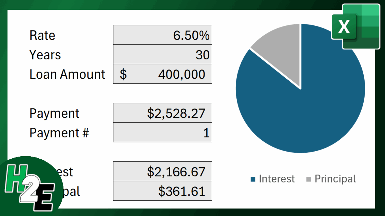
Let’s calculate the payment for a $400,000 home loan at 6.5% interest for 30 years.
1. Set up your cells
It is best to list your variables in cells rather than typing them into the formula. This makes your calculator dynamic, allowing you to just change a cell and having the result update automatically. Let’s suppose the following values are in each cell:
- B1 (Rate):
6.5% - B2 (Years):
30 - B3 (Loan Amount):
$400,000
2. Enter the PMT Formula
In payment formula, enter the following:
=PMT(B1/12,B2*12,-B3)
Notice the dash in front of B3. In accounting terms, money coming to you (the loan) is positive, and money leaving from you (the payment) is negative. By putting a negative sign before the Loan Amount, Excel returns a positive monthly payment. This is necessary to ensure that amount is calculated correctly.
3. The Result
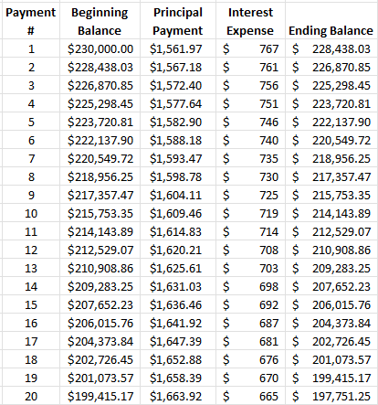
The formula will return a value of $2,528.27. This is the monthly payment which includes both principal and interest. This is the amount that will need to be paid on a monthly basis to ensure that your balance is paid off at the end of the term.
Calculating the total interest and principal portions
If you want to see exactly how much of that first payment is just the interest vs. the amount that goes towards paying off the house (the principal), you can use the following two functions:
- Interest Portion:
=IPMT(Rate/12, Period, Years*12, -LoanAmount) - Principal Portion:
=PPMT(Rate/12, Period, Years*12, -LoanAmount)
For the first month of our example:
- Interest: $2,166.67
- Principal: $361.61
Pro Tip: Since the arguments are the same, you can copy and paste the same formula and just change the function name, changing from an I to a P, so that IPMT becomes PPMT. The above example pertains to the first period, so the period argument would be set to 1. But if you want to calculate the interest or principal portion of the 10th payment, you would change the period argument to 10.
Calculating the cumulative interest and principal portions
You can also calculate the entire amount of interest and principal you’ll pay over a loan period, without having to build out an entire amortization table. Instead, here you can use the CUMIPMT and CUMPRINC for the interest and principal payments, respectively.
For the CUMIPMT formula, the arguments are similar, with the key difference being you are setting a starting and ending period. You can specify during which periods you want to calculate the interest for, but you can also just selecte everything, such as in the example below:
=CUMIPMT(B1/12,12*B2,B3,1,360,0)
The starting period is 1 and the last one is 360 (i.e. 12 x 30 years). This produces a result of $510,177.95 in total interest cost for the duration of the loan.
As for the principal, the formula is the same, with the main difference just being the function name:
=CUMPRINC(B1/12,12*B2,B3,1,360,0)
This results in a value of $400,000, which coincides correctly with the entire loan amount, as after period 360 we would expect that the entire principal has been paid back. By using these two functions, it puts into context just how much you’re paying in interest versus principal, without having to create an entire amortization table.
Free template to download
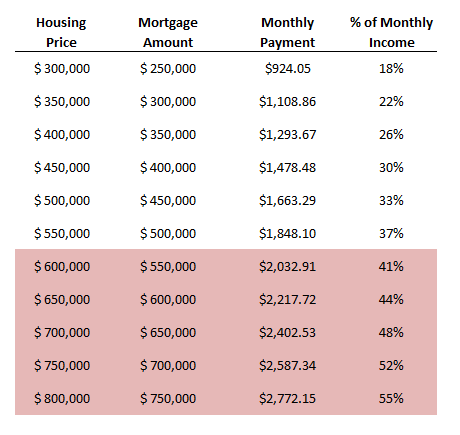
Although it isn’t terribly difficult to do these calculations once you’re familiar with the formulas, you can also just use this free mortgage payment calculator template that I’ve created. It’s easy to use an includes a sensitivity analysis, making it easy for you to look at various scenarios.
If you liked this post on How to Calculate Your Mortgage Payment in Excel, please give this site a like on Facebook and also be sure to check out some of the many templates that we have available for download. You can also follow me on X and YouTube. Also, please consider buying me a coffee if you find my website helpful and would like to support it.