How to Calculate APR in Excel

The Annual Percentage Rate (APR) on a loan tells you what your total borrowing cost is per year. It’s different from just the interest rate because it will include other expenses and fees relating to a loan. And for that reason, the APR will be higher than the interest rate. If there are no additional fees, then it will be the same. In this post, I’ll show you how you can calculate APR in Excel and how it compares with just the interest rate itself.

Functions used to calculate APR in Excel

In order to calculate APR in Excel, there’s a simple function that can allow you to do that quickly and easily; there’s no need to draw out and complicated formulas for APR that you might find online. The key is to just determine your inputs and the variables you will be using for the calculation.

The RATE function in Excel will take care of the calculation but it requires the following inputs:

• Number of periods
• Payment amount
• Present value
• Future value

The only one of these that may require some additional work is the payment amount. However, there’s also a function for that too, called PMT.

Calculating APR using an example

I’ll illustrate how you can calculate APR in Excel by using an example. Suppose you’re taking out a loan for $200,000 where you’ll incur financing fees of $30,000. The interest rate will be 4% and term is 10 years. And payments are made on a monthly basis.

For starters, we need to calculate the monthly payment amount. That requires similar inputs to the RATE function except instead of a payment amount, we need the interest rate. And since payments are going to be made on a monthly basis, both the interest rate and the term needs to be expressed in months. Instead of 4%, the rate we’ll need to use is 4%/12 and the term will be 120 months.

The PMT formula will look as follows:

=PMT(0.04/12,120,-200000,0)

Instead of entering in the interest rate to the decimal point, I’ve left it is a fraction so that the calculation is more precise. The present value is entered as a negative since the 200,000 is what is currently owed, while the future value (0) is what it will be when the loan is paid off.

The result of this calculation results in a monthly payment amount of $2,024.90.

In this scenario, there are no finance charges included. To factor those in, simply change the present value to -230,000. By doing that, you’ll arrive at a monthly payment amount of $2,328.64.

Using those payment amounts, we can now calculate the APR, using the RATE function:

=RATE(120,2024.9,-200000,0)*12

The result of this formula is multiplied by 12 to get to annual rate. This is because the RATE function gives you the rate per individual period. At the monthly payment of $2,204.90 (i.e. when there are no financing charges), the formula for APR results in a value of 4%, which is equivalent to the interest rate. Since there are no additional fees here, it makes sense that the percentages are the same.

However, when using the higher payment amount for the loan that includes finance charges, there will be a more noticeable difference. For that calculation, the formula is as follows:

=RATE(120,2328.64,-200000,0)*12

What you’ll notice here is that while the payment amount has changed, the loan remains the same. This is because while we need to pay for the extra finance charges and they are added to the monthly payment, the value we would be receiving remains just $200,000. Through this calculation, we arrive at an APR of 7.06%.

The higher the additional fees and charges, the bigger the delta will be between the APR and the interest rate.

Creating the amortization tables

The differences in these rates can also be demonstrated through an amortization table to show how the loan is paid off. For an amortization table, we need the following fields:

• Payment #
• Beginning Balance
• Principal Payment
• Interest Expense
• Ending Balance

The beginning balance will be the total that needs to be paid off. The interest expense is the calculated by taking the balance and multiplying it by the interest rate. What’s left over from the monthly payment goes towards the principal. How much is paid off is reduced from the beginning balance to arrive at the ending balance. Here’s how the table will look in the first scenario, where there were no additional finance charges:

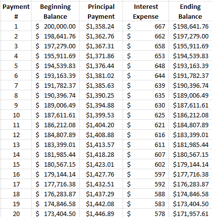
This excerpt shows the first 20 payments. The following is the amortization table for the second scenario, where finance charges total $30,000:

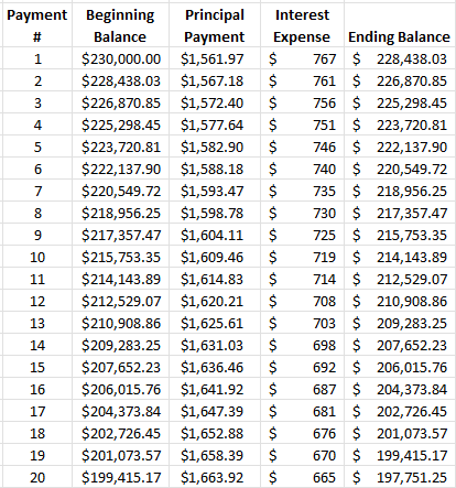
Here you can see that with a higher balance, more of the payments are going towards interest at the start. Although it takes the same amount of time to pay off the loan, higher payments are necessary to account for the increase in the beginning loan amount.

If you like this post on How to Calculate APR in Excel, please give this site a like on Facebook and also be sure to check out some of the many templates that we have available for download. You can also follow us on Twitter and YouTube.