How to Avoid Using Nested IF Statements in Excel

Nested IF statements aren’t always the most efficient way to structure your formulas. And they can make it difficult later on if you need to fix a formula or make a change to it. What’s worse, is if you inherit someone’s spreadsheet and try to dissect their nested IF functions. In this post, I’ll show you how you can get around using nested IF statements and the different alternatives you can use.

How nested IF statements works

To start, let’s look at how you might construct nested IF statements. Here’s a data set that has different cardholders and their related expenses:

I’m going to create a column with a series of IF statements to see how much Bob spent on home repair since the start of 2021. With a nested IF statement, I might first check if the cardholder is Bob. Then, if that’s true, check if the category is Home Repair. And then, check if the date is after Jan 1, 2021. Here’s how that would look inside of a formula:

=IF(B2="Bob",IF(D2="Home Repair",IF(A2>DATE(2021,1,1),E2,0),0),0)

You can see this starts to get pretty messy. And the IF statements could continue going on if you have even more criteria you want to fit into here. If I were to copy this formula down, I could get a total of all the values where Bob spent money on Home Repair. However, this wouldn’t be terribly efficient.

You could use a pivot table to quickly summarize the data by cardholder spending and category. But for this example, let’s assume that you need to do it within a formula and can’t rely on creating a pivot table when doing these types of calculations.

Using the AND function to group multiple criteria

An effective option in making your nested IF functions shorter is by using the AND function. It allows you to put all your conditions in one neat formula that you can embed within an IF function. Within the AND function, I can enter all these arguments:

AND(B2="Bob",D2="Home Repair",A2>DATE(2021,1,1))

You can keep on adding to conditions to the AND function for as many rules as you’d like to apply. This can make it cleaner to see all your criteria. All of the criteria within the AND function need to be met for the formula to return a TRUE value. Similarly, you can use the OR function if you want to check if any criteria are met.

The above formula can easily be embedded within the IF function as follows:

=IF(AND(B2="Bob",D2="Home Repair",A2>DATE(2021,1,1)),E2,0)

This does the same job as the nested IF formula except it’s a lot cleaner. However, the drawback here is that like with the nested IF statement, if you wanted to calculate all of the instances where Bob spent money on Home Repair, you would need an extra column and ad all the values up. That’s still not very efficient.

Using an Array function

Another option you can use for quickly tabulating these results is by using an array function. This can apply the logic to every cell and calculate the total for you. Rather than IF and AND statements, you can evaluate each argument, force a 1 or 0, and then multiply that by the amount to arrive at a total. Here’s how that formula might look:

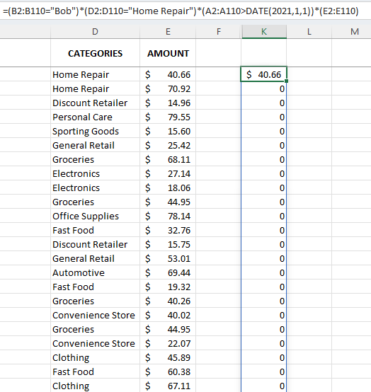
=(B2:B100="Bob")*(D2:D100="Home Repair")*(A2:A100>DATE(2021,1,1))*(E2:E100)

This formula extends to the bottom of my data set. How it works is that each group of parentheses represents an argument. If it evaluates to TRUE (i.e. the criteria is met) then the value becomes a 1. If the criteria is not met, then it evaluates to a 0. So if all the criteria is met, the results will be 1*1*1 multiplied by the amount in column E. If any one of the conditions is not met, then the result will be a 0. This is the same method as the earlier examples.

The downside of an array is that it will automatically extend to the bottom of the data set:

This again runs into a similar limitation where your formula of using up more cells than you might want to occupy. But to get around this, you could add the SUM function before your array formula:

=SUM((B2:B110="Bob")*(D2:D110="Home Repair")*(A2:A110>DATE(2021,1,1))*(E2:E110))

Using SUMPRODUCT

Another function that can do the job is SUMPRODUCT. With this function, it can take care of all the criteria while also summing up the total in just one cell. The logic is similar to how the array formula was calculated above. The key difference here is to put that all within the SUMPRODUCT function. Here’s how it looks:

=SUMPRODUCT((B2:B110="Bob")*(D2:D110="Home Repair")*(A2:A110>DATE(2021,1,1))*(E2:E110))

This will obtain the same result as if you were using the array function. SUMPRODUCT is used for multiplying arrays but it can be made to work in this fashion as well. The key is making sure you encompass all the arguments withing parentheses (hence why I opened and closed SUMPRODUCT with not one but two parentheses.

As you can see, there are many different ways you can make your formulas more efficient in Excel without having to rely on nested IF functions.

If you like this post on How to Avoid Using Nested IF Statements in Excel, please give this site a like on Facebook and also be sure to check out some of the many templates that we have available for download. You can also follow us on Twitter and YouTube.