free Archives - HowtoExcel.net

Free Credit Card Payment Calculator

October 23, 2023

by howtoexcel free free template personal finance template

Staying on top of your credit cards is an important goal when trying to get from out of debt. A credit card payment calculator is a valuable tool that can help you do just that, helping you to become debt-free sooner. The credit card payment calculator template I’ll go over in this post is free and user-friendly as well, designed to be simple to use, even for novice Excel users.

How to use the credit card payment calculator

The credit card payment calculator template in Excel is designed to provide a clear picture of your credit card debt and help you with developing a strategy to pay it off. All the fields in yellow require user input:

For the monthly payment, you need to enter at least a minimum balance. This is if you plan to pay the same amount every month. You can also specify a percentage of the balance you want to pay down each month. However, if you enter a percentage, you’ll also want to enter a minimum. Otherwise, your balance will never end up going to zero.

What’s new in this template compared to the previous version of the calculator are a couple of things. The first is the ability to add an extra payment:

Adding an extra payment to the credit card payment calculator.

As with the yellow input fields, you can enter any one-off payments in the extra payment field. This will get applied directly to your balance and reduce your principal. It will also update the rest of your payment schedule.

Another new feature of this template is the ability to enter a goal for when you want to pay the credit card off by:

Entering a value for when you want to pay off your credit card debt by.

In the above example, I have entered a date of Jan. 1, 2025. And based on my starting dating of Oct. 1, 2023, it calculates that I will need to make a monthly payment of at least $344.55 to have the credit card balance paid off by that date. Now, if I go back and enter this as my minimum payment, this is what the calculator looks like:

Credit card payment calculator schedule after changing the minimum payment.

There’s only a minimal balance remaining by the end of Dec. 2024 based on the new minimum payment but it is effectively paid off by that point.

Why managing your credit card balances is important

One of the pillars of personal finance is understanding and managing debt effectively. Credit cards, while useful, can become a financial problem when not handled effectively. This calculator highlights how much in total interest you will pay based on your payment schedule, to help show just how much the debt is costing you. And the greater the debt and the higher the rate of interest, the more costly it will be.

For instance, consider a credit card balance of $20,000 with an annual interest rate of 15%. With a monthly payment of $300, it would take approximately 12 years to pay off the debt, accruing more than $23,300 in interest — that’s more than the initial balance. If you increased the payment by just $50, that would mean paying off the credit card in about 8.4 years and the interest costs would drop to $15,330. And if you paid $400 per month, you would pay off the card in less than seven years, while incurring interest costs of $11,600. You can do all these calculations right within this calculator. You can see that even with a $50 increase you can drastically speed up your repayment schedule.

Credit card debt can be a significant hurdle when aspiring to larger financial goals like purchasing a home. Lenders scrutinize your debt-to-income ratio, and a high ratio could result in unfavorable loan terms or even disqualification. By using the credit card payment calculator to expedite your debt payoff, you enhance your credit profile, bringing you a step closer to home ownership and other financial goals.

Tailoring your payoff strategy

The what-if scenario feature can be especially useful, allowing you to determine a strategy that aligns with your financial objectives so that you know how much you need to pay every month. Whether you aim to be debt-free before a significant life event or simply wish to reduce the interest burden, this calculator lays the groundwork for a well-informed plan.

The credit card payment calculator template is more than just a tool—it’s a catalyst for proactive debt management. It nudges you to think beyond the minimum payment, encouraging a more aggressive approach towards debt elimination. By visualizing the impact of your payment strategy, you are better positioned to make choices that propel you towards financial freedom faster.

You can download the credit card payment calculator template here.

If you like this Free Credit Card Payment Calculator template, please give this site a like on Facebook and also be sure to check out some of the many templates that we have available for download. You can also follow me on Twitter and YouTube. Also, please consider buying me a coffee if you find my website helpful and would like to support it.

Get Trending Stocks Into Excel Using Power Query

June 20, 2023

by howtoexcel free free template investing power query stocks template

In the fast-paced world of investing, identifying trending stocks in Excel can provide a valuable edge for investors seeking profitable opportunities. Fortunately, with the power of Excel’s Power Query and the ability to connect to a website’s API, accessing real-time data and uncovering trending stocks has become more accessible than ever. In this article, I will go through the process of using Power Query to connect to a website’s API and importing in trending stock information.

Why should investors try to identify trending stocks?

As an investor, it is crucial to identify trending and popular stocks for several reasons:

Profit Potential: Trending and popular stocks often have significant profit potential. When a stock is gaining popularity, it usually attracts more investors, leading to increased demand and potentially driving up the stock price. By identifying these stocks early, you can position yourself to benefit from the price appreciation and generate higher returns on your investment.
Liquidity: Popular stocks tend to have higher liquidity, meaning there is a larger pool of buyers and sellers in the market. This liquidity allows you to enter and exit positions more easily, ensuring that you can buy or sell shares without significantly impacting the stock’s price. Investing in liquid stocks provides flexibility and reduces the risk of being unable to execute trades at desired prices.
Market Validation: The popularity of a stock often reflects positive market sentiment and investor confidence. When a company is trending and gaining attention, it may indicate that the market believes in its growth prospects and overall performance. By identifying such stocks, you can align your investment choices with market sentiment and increase the likelihood of investing in companies with strong fundamentals and future growth potential.
Information Availability: Popular stocks generally attract more media coverage, research reports, and analyst attention. This increased coverage provides you with a wealth of information and analysis to make more informed investment decisions. You can leverage these resources to understand the company’s financial health, competitive position, industry trends, and other relevant factors that can impact the stock’s performance.

How to get trending stocks in Excel

To get trending stock data into Excel, you should start with finding a good source that you can rely on for trending data. For this example, I’m going to use apewidsom.io, which provides free access to its API using the following url: https://apewisdom.io/api/. Here’s how I’m going to use that to pull in trending data:

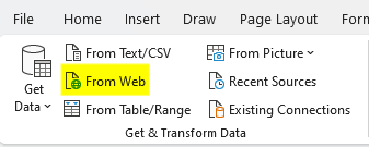
Extract the data using Power Query. To get started, I’ll select the Data tab in Excel and click on the From Web option.

Select the From Web option in Get & Transform Data to set up Power Query so that it connects to a certain web page.

Next, there will be a field to enter the URL, this is where I will paste the link that the API references:

https://apewisdom.io/api/v1.0/filter/all-stocks/page/4

Entering a URL in the From Web field for creating a Power Query connection.

After clicking OK, Power Query will launch. When the screen opens up, the following table appears. I click on List to open up another table.

After clicking that, there’s another list of records.

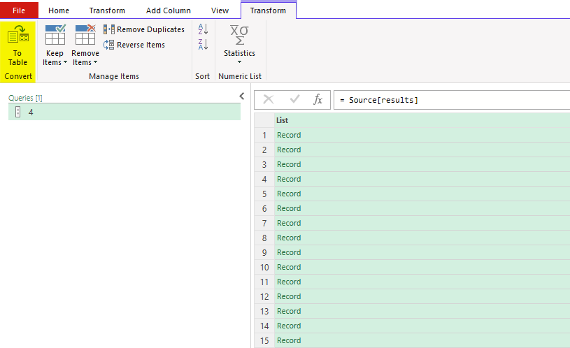
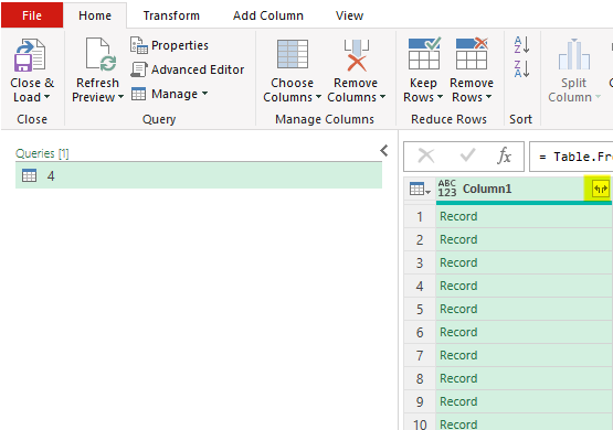
Here, I’ll select the option to convert to table and leave the default settings and click OK. Then, there is another list of records. Clicking on the button with the arrows going in opposite directions will expand them:

Expanding a list of records in Power Query.

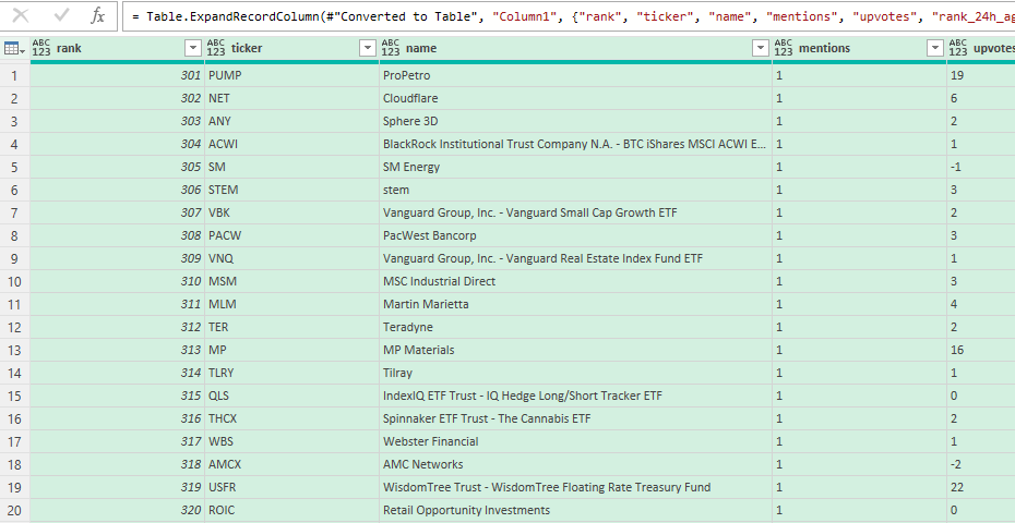
After expanding out those records, the table will now looks like a list of stocks and metrics relating to mentions, upvotes, and overall rank popularity:

Power Query table showing a stock's populating by mentions and upvotes.

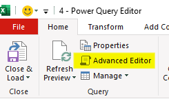
Now that this has been setup, I will convert this into a Power Query function. To do that, I’ll click on the Advanced Editor button:

Selecting the advanced editor option in Power Query.

In the editor, I will add a line at the top to specify the name of the function. And at the bottom, I will add a line to circle back to it. Lastly, I’ll add a variable for the URL as well, and put that where the link used to be:

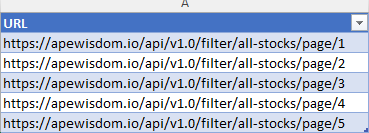
Next, with the custom function created, I’m going to go back into Excel and create a list of all the URLs I want to use this function on. In this situation, I’m going to adjust the page number at the end of the URL so that I have pages 1 through 5:

I’ll load this table, called URLtable, into Power Query using the From Table/Range button when selecting data. Next, I’ll select the Add Column tab and select Invoke Custom Function:

Selecting the option to Invoke a Custom Function.

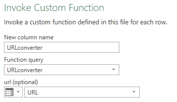
Then, I reference the query as well as the URL variable that is to be used:

Selecting which custom function to invoke.

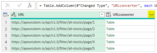
Then, there will be a field with the results, in table format. Again, this needs to be expanded out:

A list of results in Power Query after invoking the custom function.

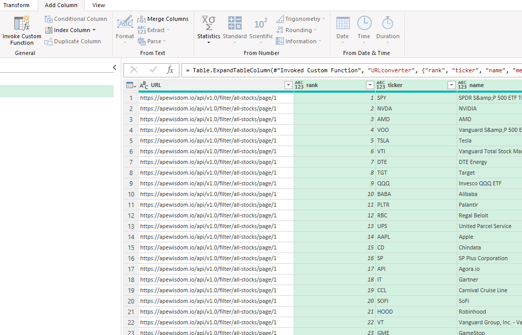
That will leave a list of stocks starting from page 1 all the way through page 5. You can remove the URL field, which is no longer needed:

A Power Query table showing the list of popular stocks.

If you don’t want to follow through all those steps yourself, you can download the template I’ve created here.

If you liked this post on Get Trending Stocks Into Excel Using Power Query, please give this site a like on Facebook and also be sure to check out some of the many templates that we have available for download. You can also follow me on Twitter and YouTube. Also, please consider buying me a coffee if you find my website helpful and would like to support it.

Free Project Tracker Template in Excel

March 3, 2023

by howtoexcel free template

If you do work on a lot of different projects, this is a template that can make your life a lot easier. It’s one that I use regularly that helps me accurately track my time. It will allow you to set up a list of different projects, and just by using a couple of buttons, you can specify when you started and stopped working on them. Whether you want to ensure you’re billing your time effectively or you just want to better manage your time and review your productivity, this template will help you do that.

How the template works

This template has two tabs: Summary and Data. You’ll first need to add your projects in the Summary tab. This will populate your drop-down list for the project field when entering data. Once you’ve updated the project list, you can go to the Data tab and start entering in data.

Entering data in the project tracker template.

You select the project, and for the details, enter a description for your task. Then, click on the green Start button. That will create a timestamp. I suggest saving the file at this point just to make sure that in the event Excel or your computer crashes, you don’t lose the timestamp. And then, when you’re done working on the task, click on the red End button. That will create another timestamp, and then it will add it to the table below. Since the file uses timestamps, you don’t need to keep it open as you work on your task.

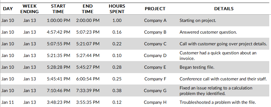
Project tracker template showing entries of tasks that have been done.

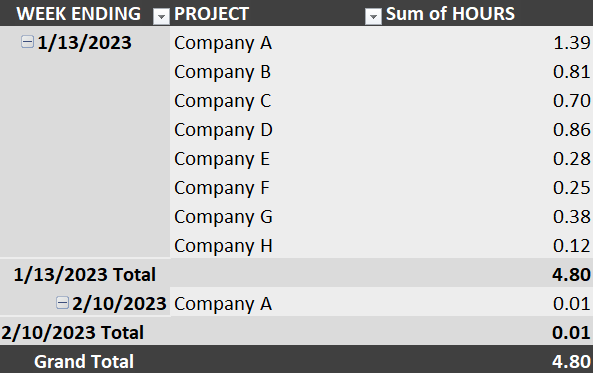
As you add entries, this table will expand. You will have the details by day, summarized by week, and it will also show you the hours spent on the task. On the Summary tab, you’ll have a pivot table that when you refresh it, will give you a summary of the time you spent both by project and by week:

Pivot table showing time spent by project per week.

Download the file

The project tracker template is completely free to use. Feel free to contact me if you have any comments, suggestions, or feedback on the file.

If you liked this Project Tracker Template, please give this site a like on Facebook and also be sure to check out some of the many templates that we have available for download. You can also follow us on Twitter and YouTube.

Mortgage Payment Calculator Template

February 10, 2023

by howtoexcel free template

Are you planning to buy a home? With this mortgage payment calculator template, you can do different what-if scenarios to see what your monthly payment will be. You can adjust interest rates, home prices, and downpayment amounts. The template will do a sensitivity analysis for you based on those variables.

How the mortgage payment calculator template works

There are eight cells that are highlighted in yellow on the template. These are all the values that you can change.

Inputs for the mortgage payment calcultor

You can specify the house price you want to start from, and the increments you want to jump by. The same fields exist for interest rate. You can also specify the term of the mortgage and your downpayment amount. There’s a space for rental income as well, in the event you plan to rent out part of your home. And lastly, there’s a monthly budget. By entering in this, the template will calculate what your maximum house price will be. This shows up in the cell that is highlighted in grey.

Once the inputs are filled in, you’ll see a range of values below. This shows you the different monthly payments at different house prices and interest rates. The beginning interest rate which you entered shows up in the middle. That way, you can see what the impact will be if interest rates are both higher or lower. If you want to see larger jumps in the house prices or interest rates, simply adjust those variables.

Conditional formatting is also used here to show you where the lowest values are (green) versus the higher ones (red).

Schedule of monthly mortgage payments with conditional formatting applied to show high versus low values.

Downloading the template

This template is entirely free to use. You can download it from here.

You may also be interested in the web-based mortgage payment calculator that’s available on this site. That too, will show you what your monthly mortgage payment will be as interest rates change.

If you liked this Mortgage Payment Calculator Template, please give this site a like on Facebook and also be sure to check out some of the many templates that we have available for download. You can also follow us on Twitter and YouTube.

Free World Cup 2022 Prediction Template and Schedule

October 11, 2022

by howtoexcel with No Comment free free template template

The World Cup is starting next month and I have a free template for you to use whether you want to track the matches or make predictions with a group of friends. The entire schedule is downloaded within the file, and you can enter the the scores — both actuals and predictions.

How the template works

There are four tabs on the template:

Actuals: This sheet name needs to remain intact as when comparing your predictions, this is the source data that the prediction results will compare against.

Prediction.Blank: This is a blank sheet that is the same as the actuals that you can use for making predictions.

Prediction.Results: This is where you should post your final prediction results. Column A (name) is for the name of the person whose predictions they are. In columns B:D, you just need to copy those fields from the Predction.Blank page for any predictions you or someone else makes. It’s important the values are in the correct fields for everything to be recorded correctly. Also, make sure to paste them as values to ensure the formulas aren’t being copied over.

I’ve also added a section below the main prediction table that shows the teams you predicted to advance to each elimination stage:

This should also be copied over to the Prediction.Results tab. The stage should go in column B and the team will go in column C. I’ve left an example of how the Prediction.Results tab should be filled in within the template so that you can follow along. The table will automatically calculate and compare against the actuals.

Scoring.Rules: Here you can set up how points are allocated if the score, result, and total number of goals are correct. You can also specify if the teams need to be correct (applicable for knockout rounds) and how many points to assign if you’ve got the right team in the right elimination stage.

The basic idea is that you can make a copy of either the Actuals or Prediction.Blank sheet and give to someone to fill in. Once you get back their predictions, you can paste them into the Prediction.Results table. Then, once the tournament begins, you populate the Actuals. After that, it’s just a matter of updating the pivot table on the Prediction.Results page to see who has the most points.

Enter scores in the 0:0 format

One important item to note is that when entering scores, there should be a number followed by a colon, then by another number. There should be no spaces any no different characters, otherwise you will get an error and the value won’t be read properly.

In the case of shootouts and extra time, there is no extra field to enter these values in. For the purpose of minimizing the complexity of formulas, only one column is used for scores. The workaround for this is if a team wins in extra time or a penalty shootout, simply add 1 to their score so that instead of entering it as 1:1 (5:4) it would just be 2:1.

Tables will update automatically

The benefit of using the template is that the tables will automatically update based on your selections. This will help you in determining which teams play one another in the knockout rounds.

The template does factor in tiebreakers but in the event that a rare situation comes up where the tiebreaker doesn’t calculate correctly (e.g. it comes down to fair play points) then you have the option to override the values.

Next to the tables, there is another table for overrides:

In this example, I have overridden the results so that these will be the standings for Group B regardless of what the spreadsheet has calculated. You don’t need to list every team in a group and only need to list the teams that are tied. You also don’t need to specify the group letter.

Adjust the times for your time zone

Another feature that I’ve added here is to adjust the game times for your particular time zone. On the left-hand side you can specify how many hours you need to adjust for GMT. Remember that the value here will need to factor in for any daylight savings that may be in effect for your location (Qatar doesn’t adjust its time).

For example, in my region, my GMT adjustment is -7 but after factoring in for daylight savings in November, it becomes -8. So please remember to adjust for any daylight savings adjustment that might happen between now and the start of the tournament. For GMT -8, the local time would adjust by 11 hours (Qatar is +3), and so a match starting at 7pm local time would be playing at 8am in my time zone.

Highlight teams with a Watchlist

You can also highlight teams you want to track on the schedule by adding them to a Watchlist next to the schedule. For example, suppose I want to follow any games involving Canada and the USA:

World cup schedule shown with matches highlighted.

Any values that are entered under the Watchlist will highlight corresponding matches on the schedule. For this to work, you need to enter the team names the same way that they are spelled out on the match schedule.

Download

This template is available free of charge, and you can download it here. It is locked to ensure that the formulas remain intact and nothing gets accidentally erased or overwritten.

If you like the Free World Cup 2022 Prediction Template, please give this site a like on Facebook and also be sure to check out some of the many templates that we have available for download. You can also follow us on Twitter and YouTube.

Free Excel Template to Track Berkshire Hathaway’s Portfolio

September 13, 2022

by howtoexcel with No Comment free free template investing stocks template

Warren Buffett fans like to track the billionaire investor’s moves, and a good way to do that is through Berkshire Hathaway’s 13f filings. His company reports its holdings every quarter, showing where there were changes in its positions. By looking at multiple filings, investors can track the changes from one period to another. With this free template, you can do that quickly and easily all on your own. All you have to do is specify the specific filings that you want to compare to one another.

How the template works

This template uses PowerQuery to grab the data from the 13f filings. It will then compare the two to find the changes in share count.

There are only two inputs you need for the template, both are on the Current.Holdings tab. You’ll need to paste the URL for the current 13f filing and the previous one (or whichever filings you want to compare against one another). It can sometimes be a bit tricky to get exactly what you’re after. Here’s how you can find the 13f filings for Berkshire Hathaway to use in this template:

Click on the following link, which has company’s filings on the SEC website: https://www.sec.gov/edgar/browse/?CIK=1067983 (this link is included within the template).
Click on the View filings button on the page.
Do a search for 13f so that you can see just the 13f filings on that page:

Berkshire Hathaway's 13f filings on the SEC website.

4. Find the reporting period you want and click on the Filing button — don’t click on the actual description next to it.

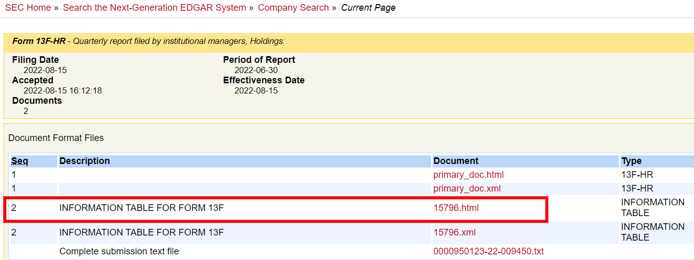
5. When you open up the link, you should see multiple files you can open. Select the information table that is in html format:

Selecting the information table in HTML format from the SEC website.

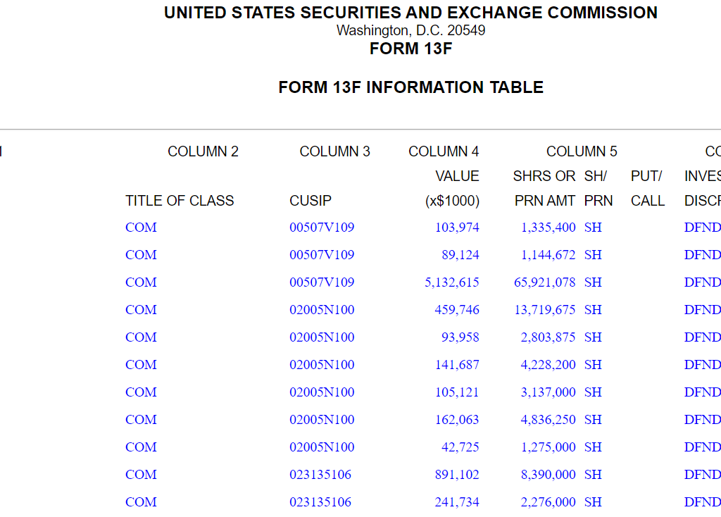
When you open the file, you should see the holdings in a table format:

If this is what you see, then the link you’ve downloaded will work. Note, on older 13f filings (e.g. 2013 and older), the format is in a text file and they won’t work with this template.

6. Copy the link and enter it into one of the fields on this template, either for the new filing or the old one.

Entries for the old and new 13f filings.

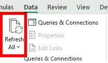
7. Once you’ve filled in both the new and old links, then go to the Data tab in Excel and click on Refresh All. This will update the queries that the template relies on, and calculate the changes.

Now the different sheets will update:

Current.Holdings: this will show you the current holdings as per the New13f file
Change.In.Holdings: this will show you the change between the two filings. The change will be reflected in total shares and as a % of change in shares.
Old.Holdings: this will show the number of shares held per the Old13f file.

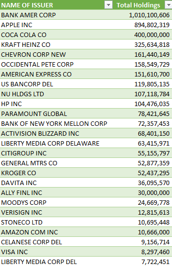
Summary of Berkshire Hathaway's holdings per their latest 13f filing.

Download the template

This template is completely free to use and you can download the Berkshire Hathaway 13f Template here.

If you like the Berkshire Hathaway 13f Template, please give this site a like on Facebook and also be sure to check out some of the many templates that we have available for download. You can also follow us on Twitter and YouTube.

Manage Your Subscriptions With This Free Template

July 26, 2022

by howtoexcel with No Comment free template vbafree

Nowadays, everything is available on a subscription. Even BMW now offers heated seats on a recurring subscription. It can be a challenge to keep on track of all your subscriptions, including when they renew and when trials end. However, I have a free template just for these purposes. With my free template, you can stay on top of your subscriptions and see just how much you are spending on them on a monthly and annual basis.

How the subscription manager template works

This template has no macros and is designed to be easy to update and track. Here’s how it looks:

There are multiple charts to show you the annualized cost of your subscriptions and the monthly cost (which is shown by category). This can be effective for budgeting purposes to know how much all of these subscriptions are costing you.

To add a subscription, simply add it to the bottom of the table. You can enter a category name, a frequency, amount, as well as subscription and renewal dates. The columns that have headers highlighted in grey don’t need to be updated as there are formulas there. This is where the amounts for the monthly and annual costs get calculated. Whether your subscription is paid monthly or annually, these columns will work out the calculation to determine what it costs you both on an monthly and annual basis. That way, you don’t need to worry about grouping monthly and annual subscriptions separately.

There’s also another column called Days to Action — this will calculate the days between today’s date and the renewal date. It will highlight in yellow when you are within 30 days of the renewal date, and it will turn red when you’re within two weeks of it. The point here is to give you a warning that a renewal is coming up (or a trial is ending). This can help you prevent forgetting about it and incurring a surprise fee. If you don’t care to track this, you can just leave the renewal date blank.

Updating the data in the template

When you enter a new line for a subscription or want to make modifications to one, the charts won’t automatically update as there are no macros within the file. In order to trigger an update, go to the Data tab and click on the Refresh All button. Upon doing so, your charts will be updated.

If you want to remove a subscription, simply right-click on the row and delete it. If you’re within the table, then while you’re on the row, right-click and select Delete. You’ll see an option to remove Table Rows. Either method will work fine.

Download the subscription manager template

The subscription manager template is available here

If you like the Subscription Manager Template, please give this site a like on Facebook and also be sure to check out some of the many templates that we have available for download. You can also follow us on Twitter and YouTube.