dates – Page 2 – HowtoExcel.net

Free Excel Date Picker Add-In

May 18, 2021

by howtoexcel with No Comment add-ins dates macros

Are you looking for an easy way to add a date to your Excel spreadsheet? You can download my free date picker add-in for Excel. It is useful if you have a form and you want people to select dates or if you just want an easy way to enter a date without worrying about whether it is in the right format.

***Please note on an earlier version of this add-in (and as reflected in the video), the calendar was designed to pop up next to the active cell. However, due to many issues related to scrolling and possible zooming, and multiple screens, it is now set to open at the top (and in the middle) of the screen***

How the date picker add-in works

To launch the add-in, click on CTRL+SHIFT+Z, which will trigger the following calendar to pop up:

By default, it will jump to the current month. Clicking on any of the dates will enter the date value into the active cell. You can use the arrow keys on the left or right side to change the months. If you want to jump by years, double-click on the year and just enter the desired year. The calendar will automatically adjust, which will be quicker than if you were to just continue pressing the arrow buttons.

Right now the add-in is a stand-alone but look for it to be included as part of a larger add-in package. If you have any suggestions for other features to include in an add-in, feel free to contact us.

How to install an add-in

You can download the date picker add-in here. Once you’ve saved it, go into Excel and select File -> Options -> Add-ins and then depending on your version, you may see an option at the bottom to go to manager Excel Add-ins:

Click on the Go button and then you will have a list of add-ins you can install. If you didn’t save the add-in into the default folder where the rest of the Excel add-ins are, you just click the Browse button to find where you saved the file. Then, make sure the add-in is checked off and click OK and it will be ready to go.

If you liked the Date Picker Add-in, please give this site a like on Facebook and also be sure to check out some of the many templates that we have available for download. You can also follow us on Twitter and YouTube.

Calculate Hours and Minutes Between Two Times

November 21, 2020

by howtoexcel with No Comment dates intermediate tips & tricks

Do you want to know how to calculate how many hours and minutes have elapsed between two times? Below, I’ll show you how to do that with Excel formulas. The difference won’t be in just fractions of days or hours but real minutes and hours that make it easy to measure. To make this work, however, the first step is entering in the time correctly.

How to enter time in Excel

Excel has a built-in time function called TIME where you can enter the hour, minute, and second. For example, if you wanted to enter a time of 6:30 AM, you could enter a formula of TIME(6,30,0). Alternatively, you could type in 6:30 AM — the key is leaving the space between the time and the AM/PM indicator.

However, the one clear limitation here is that this won’t help you if you want to calculate the hours and minutes between times that span more than just one day. By using the TIME function, or entering just the hours and minutes, Excel is always going to assume you’re talking about the current day.

The best way to enter in time is to also factor in the date. Depending on your regional settings you might enter this differently, but this is how I’d enter a time of 8:00 PM on Nov. 20 on my computer:

2020-11-20 8:00 PM

I can also use a 24-hour clock and type in the following:

2020-11-20 20:00

Either way, Excel knows what time I’m talking about. If you always want to return the current time, you can use the NOW function.

For the start time, I’ll set it to the start of the year: 2020-01-01 0:00

Calculating the difference

Just using the minus operator, I can get the difference between these two dates as follows:

By default, Excel will return the number of days, including the fractional days as well. To convert days and calculate the hours instead, we will multiply the difference by 24, since that’s how many hours are in a day. That gives us the following:

That’s 7,796 hours between those two dates and times. It’s a nice round number but what if we changed it so that the end date was at 8:30 pm, or 20:30, this is what the updated calculation would look like:

Now I’ve got that residual 0.50 which indicates half an hour. But I want minutes, not fractions of an hour. The easiest way to do this is to create one calculation for hours, and another for minutes. Then, afterwards, you can concatenate them together. To get the total hours, I’ll adjust my formula to include the ROUNDDOWN function so that it does not include the 0.5. It looks something like this:

=ROUNDDOWN(datedifference*24,0)

Where datedifference is that raw calculation between the two dates and times. In my calculation, I’m still multiplying the time difference by 24 to get to hours, and then I round that to 0 spots, which is indicated by the 0 in the second argument. Now it will only show 7,796.00 for hours.

To calculate the number of minutes, I’ll need to multiply the datedifference by 24 and then again by 60, to convert the difference into minutes. This is what my calculations look like thus far:

My hours are nicely rounded but my minutes include the total minutes, which is not what I want. I only want the minutes that are left over after the hours are factored out. Here I can make use of the MOD function which will tell me the remainder after division. I’ll adjust the minute calculation to calculate the remainder after I’ve divided the total minutes by 60. This will determine what’s left over after pulling out full 60-minute hours, which is that residual 0.50 that I’m after. Here’s what this formula looks like:

=MOD(datedifference*24*60,60)

That gives me the following result for minutes:

Now I get a nice and round 30 minutes. There is the potential that I can also get partial minutes if I have seconds in my calculation. This could be the case if I’m using the NOW function. To correct for this, I can again use the ROUNDDOWN function as I did for hours.

However, let’s assume that you also want to track seconds. We can do that as well. I’ll break out another column for seconds. There, I’ll multiply the difference by another factor of 60, to get the following:

Time difference in hours and minutes and seconds.

I added 25 seconds to my end date, which is why you’ll notice there’s a slight change in the difference column from this screenshot and the earlier one. Right now, total seconds tells me there are 28,067,425 seconds between these two times. If I want to get the raw number of seconds, then I’ll again use the MOD function and again use 60 as a divisor, since now I want to factor out the minutes:

I now have a clean breakdown between hours, minutes, and seconds between these two times. But if you want to calculate more than just hours between two times, you can also incorporate the number of days as well.

Breakdown of days, hours, minutes, and seconds

If I wanted to take a different approach and break the difference down by days, and then by hours, minutes, and seconds, I’ll first need to break out the days. Since that’s the default calculation for Excel, all I need to do is use the ROUNDDOWN function on the difference. The formula is as follows:

=ROUNDDOWN(difference,0)

And that gives me this:

If I wanted to get the hours that are remaining, what I can do is take the difference, use the MOD function, but this time I’m using a divisor of just 1, since I really only want the decimal place after the full number. Then I’ll multiply that by 24 hours, and again, use the ROUNDDOWN function:

=ROUNDDOWN(MOD(difference,1)*24,0)

Now my hours total looks like this:

I’ve got a nice round 20 hours, which makes sense since 8:00 PM is 20:00 on a 24-hour clock. To calculate the difference in minutes, I can revert back to the earlier calculation where I used the MOD function to determine what’s left over after multiplying the difference by 24 and 60, and then dividing it by 60 minutes:

Time difference in days, hours and minutes.

The seconds calculation will work the same way as well. The only difference in the way to break out hours and days was to adjust the hours calculation to ensure it isn’t taking in the full hour difference, only the residual amount that pertained to the current day.

Now that you’ve got all the chunks broken down between days, hours, minutes, and seconds, you could concatenate that into one large formula, Something like this might work:

=CONCATENATE(daydifference,” Days “,hourdifference,” Hours “,minutedifference,” Minutes “,seconddifference, ” Seconds”)

That produces the following:

For this not to be a messy result, you’ll want to ensure you’re using the ROUNDDOWN function in each of those calculations so that you aren’t keeping any trailing numbers.

If you liked this post on how to calculate hours between two times, please give this site a like on Facebook and also be sure to check out some of the many templates that we have available for download. You can also follow us on Twitter and YouTube.

How to Make a Countdown Timer in Excel

May 23, 2020

by howtoexcel with No Comment dates macros template vba

A countdown timer can help you track how much time there’s left to do a task or until a deadline comes due. Below, I’ll show you how you can make a countdown timer in Excel that can track days, hours, minutes, and seconds. In order to make it work, we’ll need to use some VBA code, but it won’t be much. And if all else fails, you can just download my free template at the end of the post and repurpose it for your needs.

Let’s get right into it and start with the first step:

Calculating the difference in days,

To calculate the difference between two dates is easy, as all you’re doing is subtracting the current date and time from when you’re counting down to.

The start date is just going to be today, right this very second. And Excel has a convenient function just for that, called NOW. It doesn’t require any arguments and all you need to do is enter the following formula:

=NOW()

Entering the date and time you’re counting down to is a bit trickier. As long as you enter it correctly, then calculating the differences will be a breeze. However, this may involve a little bit of trial and error since it’ll depend on how your regional settings are setup. For the countdown date, I’m going to set it to the end of the year. Let’s say 11:00 PM on New Year’s Eve. Here’s how I input that into my spreadsheet:

2020-12-11 11:00 PM

The key things to remember here are that there should be a space between the time and the AM/PM indicator (if you use it) and there should be two spaces between the date and the time. Then, it’s just a matter of whether you’ve got the right order of date, month, and year. This is where you may need to do some testing on your end to ensure you’ve got the correct order.

Now that the dates are set up, we can calculate the difference in days. To do this, we can just calculate the difference and use the ROUNDDOWN function to ensure we aren’t adding partial days:

There are 222 days left until the end of the year. By using the NOW function, the formula will automatically update and tomorrow the days remaining will change to 221, and so on. If your output’s looking a little different, make sure to check the formatting and that it’s set to days.

Calculating the difference in hours, minutes, and seconds

There’s not a whole lot of complexity when it comes to calculating the difference in hours, minutes, or seconds. We’re still subtracting the current date from the deadline. The only difference is that now we’re just going to change the formatting. If I do a simple subtraction, I end up with a fraction, which isn’t really usable in its current format:

Counting down the hours, minutes, and seconds left.

The trick here is to change the format of this cell so that it shows me hours, minutes, and seconds. And that’s an easy fix. If I just click on cell C10 and click CTRL+1, this will get me to the Format Cells menu. In here, I’ll want to select a Custom format so that the cells just shows hours, minutes ,and seconds:

Here’s what the countdown timer looks like after the format changes:

It’s important to include a date in the calculation even though we’re just doing a difference between hours, minutes, and seconds. Otherwise, the formula wouldn’t correctly calculate in all situations, such as when the deadline hour is earlier than our current hour.

Putting it all together

Now that all the calculations are entered in, now it’s just a matter of formatting the data. We can create a countdown clock that separates days remaining, from hours, minutes, and seconds remaining.

One cell can have the difference in days, while another will have the difference in hours, minutes, and seconds. This goes back to just modifying the formatting and applying a custom format. Here’s how mine looks:

Although we’ve gotten to this point, the challenge is that this countdown timer still doesn’t update on its own. Unless you want to click on the delete button all the time, the countdown isn’t going to move unless there’s something to trigger a calculation in Excel. That’s why we’re going to need to add a macro to help us do that, which bring us to the important last step of this process:

Adding a macro to refresh every second

We need a macro to update the file. Whether it’s every second, every five seconds, it’s up to you. While the countdown timer will update when someone enters data or does something in Excel, that’s not much of a countdown. This is where VBA can help us. If you’re not familiar with VBA, don’t worry, you can just follow the steps below and copy the code.

To get into VBA, click on ALT+F11. From the menu. Once you’re there, click on the Insert button on the menu and select Module:

Over to the right, you’ll see some blank space where you can enter in some code. Copy and paste the following there:

Sub RunTimer()

    If Range("C10") <> 0 Then
        Interval = Now + TimeValue("00:00:01")
        Application.Calculate
        Application.OnTime Interval, "RunTimer"

    End If
End Sub

One thing you may to change is the reference I made to cell C10. Change that to where you have your countdown timer. As long as there’s a value in the cell, the macro will continue running. All it does is check if there’s a value there, and if there is, it updates the worksheet every second. And by doing that calculation, your countdown timer will update even if you’re not making any changes to the spreadsheet.

You can also change the interval which currently updates every second, as noted by the 00:00:01. You can change this to five seconds, 10 seconds, however often you want it to update.

But there still needs to be something that triggers the macro to start running. You can assign a button or shortcut key to do that.

However, in this example I’ll activate it when the sheet is selected. Inside VBA, you should see a list of worksheets. Double-click on the one that contains your countdown timer:

You’ll again see blank space to the right where you can enter code. And you’ll also see a couple of drop-downs near the top that you’ll want to look for. By default, the first one should say (General). Change this to Worksheet:

Next, change the other drop-down which will probably say SelectionChange. Change it to Activate. Then you should see something like this:

Selecting the worksheet activate event in VBA.

Copy the following code into there to call the macro we created above:

RunTimer

Now when you switch to another worksheet and come back to the current one you’ll notice your countdown timer is updating on its own. If you want it to stop it, just clear the cell that has the timer. Otherwise, the macro will continue running every second.

The Countdown Timer Template

If you’d rather just use a template, then you can download one that I’ve made here. You don’t have to worry about macros and instead you just need to enter the end time; the time that you’re counting down towards.

I’ve also got a start/stop button that you can toggle to get the countdown timer going and that will pause it:

You can move the button as well as the time your counting down to onto another sheet if you don’t want someone altering it. If you have any questions or comments about this template, please send me an email at [email protected]

If you liked this post on how to make a countdown timer in Excel, please give this site a like on Facebook and also be sure to check out some of the many templates that we have available for download. You can also follow us on Twitter and YouTube.

How to Do a Weekly Sales Analysis and Compare the Same Days of the Week

March 7, 2020

by howtoexcel with No Comment accounting dates forecasting intermediate

Whether you’re doing a forecast or looking back at how your sales were over a period of time, it’s important to ensure that you’re comparing apples to apples. While monthly and yearly numbers won’t have too much noise, once you’re trying to do a daily or weekly sales analysis, that’s when things can get a little challenging.

Below, I’ll show you how you can do a weekly sales analysis where you’re comparing the same days of the week against one another. This will give you an accurate picture of your year-over-year performance.

Step one: determine which day of the week you want to start on

This is a simple step and you’re probably going to go with either Sunday or Monday. But it’s an important one to consider because when you’re looking at weekly sales numbers, you want to be consistent. And while you can refer to the week number when comparing one week to a previous year, saying week 32 is not going to be as useful as saying the week starting August 5 or ending August 11.

In my example, I’m going to use Monday as my starting point to ensure that I’m not breaking up the weekend (the default in Excel is Sunday). To make it easy to compare a week, it will be helpful to create a header for the days of the week so it looks like a calendar.

Step two: entering the first date of the weekday you selected

The first Monday of 2020, wasn’t until Jan. 6 this year, which would be the second week of the year if we start on Mondays. The previous Monday was Dec. 30, which was technically week 53. Weeks 1 and 53 are often abbreviated. For now, just accept that there’s no Monday in Week 1 of 2020. I’ll show you how we can get around this problem further down.

For now, Jan. 6 will be our starting point which we’ll call Week 2. Now, that we have our starting point, we can build out what our subsequent weeks will look like.

For example, if I want to find out the start date for week 40, what I can do is simply use the following formula:

First, I multiply 7 by the difference in weeks. Then, add that to the first Monday value. In this example, it tells me the 40th Monday of the year is Sep 28, 2020. That’s why setting up the first Monday values is important to ensure that it’s easy to get the remaining dates.

This is the easier approach to take. However, later on I’ll show you a way where you don’t have to enter in the first Monday of the year.

Step three: filling in the remaining dates of the week for your sales analysis

Getting the starting date of the week is the toughest part. From there, all you have to add is just add 1 to each subsequent day:

Just adding 1 to the previous date will increment to the next day. No special formulas needed here.

Step four: getting the prior-year date

To get the previous year’s data you can follow the same approach as in step two. However, I’ll use this as an opportunity to show you another way that you can get the data. One that won’t require you to pull out the calendar.

First, we need to know what day of the week Jan. 1, 2019 fell on. To do this, we can just use the following formula:

=WEEKDAY(“Jan 1, 2019”,2)

The reason I put the number 2 as the second argument is because my week is starting on a Monday. If I set it to 1 or left it blank, the default would be Sunday. This is important because if Monday is my first day of the week then it’s day value is 1 and Sunday is 7. Had I used Sunday, then Sunday would have a value of 1 and Monday would be 2. This is why it’s important to know which day of the week you want your week to start on.

In 2019, Jan. 1 fell on a Tuesday, and the formula above gave me the result of 2. (Monday is 1, so Tuesday would be 2). The reason I need to know the weekday is because I need to adjust the date to find out when that week actually started. I use the following formula to do that:

=DATEVALUE(“Jan 1, 2019”)-(WEEKDAY(DATEVALUE(“Jan 1, 2019”),2)-1)

What this formula does is subtracts Jan 1, 2019 from the number of days it is above day 1. It then moves the date back. I can simplify this formula by entering Jan 1. 2019 in cell A1. Then my formula looks like this:

=A1-(WEEKDAY(A1,2)-1))

I no longer need to use the DATEVALUE function and now it’s a bit easier to use. There’s also less chance of an error when entering the date. Now, when I want to find out the first day of the week, I can multiply 7 times the week number and add to this calculation:

=(A1-(WEEKDAY(A1,2)-1))+(7*(B1-1))

B1 is the week number. In this example, if I were to enter Jan 1. 2019 for cell A1, that would give me a result of Dec 31. 2018 for the start of Week 1. Excel also considers this to be the week that contains Week 53 and Week 1. This is where you can get around this issue. By calling this Week 1 of the current year and including December’s days into this week, it will ensure you don’t have the Week 53 problem. It may not look great to call the previous year’s dates part of the new year but it avoids having to manually make adjustments for this period.

Using the updated formula, I can change the Jan. 1 date to reflect 2019 and use week 40 to update my comparables for the weekly sales analysis:

From here, it’s just a matter of now using a SUMIF function on your data to pull the sales for each one of these dates and you’ve got your comparable sales numbers. With 2020 being a leap year, you can see that the dates have moved up two days from the prior year. Without the date adjustment, you could have ended up comparing a Sunday (Oct 4, 2020) against a Friday (Oct 4, 2020).

If you liked this post on how to do a weekly sales analysis, please give this site a like on Facebook and also be sure to check out some of the many templates that we have available for download. You can also follow us on Twitter and YouTube.

How to Remove Time From Excel Date

February 29, 2020

by howtoexcel with No Comment dates find intermediate left mid parse tips & tricks

If your data contains date and time, and you only need the former, there are ways for you to remove time from the excel date. The first step, however, is in determining whether your data is in date format or whether the information is stored as text. Depending on which one it is, it will change how you will need to manipulate the data.

You can use the TYPE function to determine whether your data is in text or numeric format. The function evaluates a value and if it is numeric it will return 1 and if it is text the result will be 2. That will determine which path you need to focus on: converting a text date or just pulling the date values that you need. The latter is the easier of the two approaches.

Removing time from a date value

If the data is in date format, then it’s as easy as using the DATE function to pull out the fields you need. Let’s start with a date that shows the following:

2020-02-29 12:00:00 PM

It has more detail than we need with the time in there but it also has everything that’s needed—year, month, and day. The easiest way to pull out the date is using a formula as follows (where A1 is where the original data is):

=DATE(YEAR(A1),MONTH(A1),DAY(A1))

The DATE function takes three arguments: year, month, and day. By pulling these values out from the cell that has the time, we’re effectively creating a new value that has everything except the time. Now, if you don’t want this to remain a formula what you can do is copy the cell with the date and not the time, and paste it as values. Now, you’re left with hard-coded date values that do not contain the time.

As mentioned, this is the easy part of the process. The more difficult one is if your date is stored as text and where the DATE function results in an error if you try the above calculation. Let’s take a look at how to remove time from an Excel date when it’s in text format.

How to extract the date from a text field

If the same value above was stored as text, the formula involving the DATE function would result in an error. To pull the values that are needed to arrive at a proper date value, we’ll need to parse the data. Parsing can be a bit complicated but when you’re dealing with text, it’s the only way around getting the data you need.

In the above example, the date fields were separated by hyphens but it could be that slashes are used as well. Ultimately, it doesn’t matter, so long as there is some pattern that separates the month, day, and year fields. We will still use the DATE function. But in order to put the correct values in, pulling out the key information is going to be the challenging part.

Let’s start with pulling out the month, since in a month-day-year format, it’ll be the first value and thus, the easiest to extract. Here’s how the formula to pull the month would look, again, assuming A1 is where the data is:

=LEFT(A1,FIND(“-“,A1,1)-1)

Since the month is the first value, we use the LEFT function to pull the characters at the beginning of the cell. A1 is the cell we’re looking at, and the second argument is the length of the string to pull. Here, we’re looking for the dash(-) within the cell and subtracting one character so that the dash itself isn’t included in the extraction. This formula would produce a value of ’02’ and correctly return the month value.

To get the day is a bit trickier since it’s between dashes. It’s still possible to extract it but the formula is a bit more complex and requires using the MID function. Here’s the function with just the first two arguments filled in:

=MID(A1,FIND(“-“, A1 )+1,

The first part of the formula specifies the starting point. For here, we’re again using cell A1 but this time we’re looking for the dash using the FIND function to indicate where the second value begins. We add one to this value to ensure that we aren’t starting at the dash. Here’s what the next argument looks like, for the length of the value:

=FIND(“-“,A1,FIND(“-“, A1,1)+1)-FIND(“-“, A1,1)-1)

Here what we’re doing is using the FIND function to search for the dash but this time we aren’t starting from the first position but are starting from where the first dash was found, and adding a one to that. Then we subtract where the first dash was found, and the difference is the length of the string. It’s a complicated, nested function but it does what we need it to do. The completed formula for the day looks as follows:

=MID(A1,FIND(“-“,A1,1)+1,FIND(“-“,A1,FIND(“-“,A1,1)+1)-FIND(“-“,A1,1)-1))

The last part is to extract the year. And because this comes after the second dash, we’re going to need to nest two FIND functions, not just one. You could try and always start from a certain number, for example, the seventh character if your date format will always by mm-dd-yyyy. However, using the FIND function ensures you aren’t taking any assumptions (e.g. they may be leading spaces). I also avoid hardcoding numbers in formulas whenever possible. Here is the formula that remains for the year function:

=MID(A1,FIND(“-“,A1,FIND(“-“,A1,FIND(“-“,A1,1)+1))+1,4)

The nested FIND functions are needed to ensure that I’m starting to search for the dash after the second instance was found. I use the number four for the last argument because rather than making this formula even more complicated, I figure the year will either be two characters or four, and it won’t deviate. If your data contains two characters for the year, then you can just change the final argument accordingly.

That leaves us with this long formula to extract the date for the mm-dd-yyyy:

=DATE(MID(A1,FIND(“-“,A1,FIND(“-“,A1,FIND(“-“,A1,1)+1))+1,4),LEFT(A1,FIND(“-“,A1,1)-1),MID(A1,FIND(“-“,A1,1)+1,FIND(“-“,A1,FIND(“-“,A1,1)+1)-FIND(“-“,A1,1)-1))

It’s a complicated one so it may be easier to just copy and paste it rather than trying to reconstruct it yourself. If your original date is in dd-mm-yyyy format, here is a formula for that:

=DATE(MID(A1,FIND(“-“,A1,FIND(“-“,A1,FIND(“-“,A1,1)+1))+1,4),MID(A1,FIND(“-“,A1,1)+1,FIND(“-“,A1,FIND(“-“,A1,1)+1)-FIND(“-“,A1,1)-1),LEFT(A1,FIND(“-“,A1,1)-1))

This just involves flpping around the formulas to grab the month and day. If your dates use “/” instead of “-“, then you can just to a find and replace in the formulas above to replace all the “-” with “/” or whatever else your system may use. Regardless how the data is separated, you can adapt the formula to how your data looks.

As you can see, having your data in the right format can make this process a whole lot easier. It’s once you get into text that it becomes much more challenging in pulling the date out. And again, once you’ve got the data you want, copying and pasting as values will ensure you don’t have to keep both the old and new data together.

If you liked this post on how to remove time from Excel date, please give this site a like on Facebook and also be sure to check out some of the many templates that we have available for download. You can also follow us on Twitter and YouTube.

How to Calculate Time Difference in Excel

January 26, 2020

by howtoexcel with No Comment dates intermediate parse

If you need to keep track of time entries, whether for a timesheet or some other purposes, it’s important you know how to calculate time differences in Excel, and that’s what I’ll show you how to do in this post. If you’re just looking for the difference in dates, including months, days, or years, then refer to this post. But if you need time differences, keep reading.

Entering time correctly

In order for the difference in time to be calculated correctly, it should ideally be entered in the right format to start with. Let’s use the example calculating the hours worked for a regular 9-to-5 shift.

You can use a 24-hour clock or AM/PM to enter time. If you’re using AM/PM, then you’ll want to make sure you enter a space between the time and the AM/PM indicator. For example: 9:00 AM rather than 9:00AM.

If you enter it correctly, then the value you just entered should align to the right. This means that Excel has interpreted it as time. You can also tell because in Excel it will show as 9:00:00 AM in the cell details. Normally, you aren’t going to enter seconds but Excel will track those extra zeroes anyway.

If you were to just enter 9AM then you’ll notice after hitting enter that nothing happens and Excel doesn’t align it to the right side of the cell. This means that what you’ve entered Excel is reading as text.

That is a problem because if you want to calculate the time difference correctly, it’ll get a whole lot more complex and require using IF and MID functions. It’s not impossible (and I’ll show you how to do so later on), but it will make it a lot more complicated.

Calculating the time difference

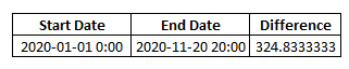
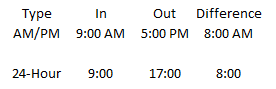
Now that you’ve made sure that the time entries are entered correctly, it’s time to show you how to calculate time difference in Excel. Here’s how it looks if I just take the end time and subtract the start time:

calculating time difference for am pm and 24-hour time

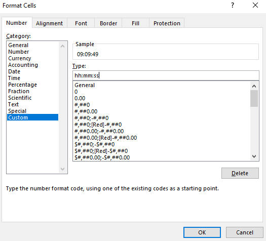
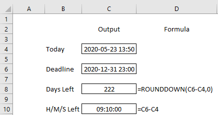
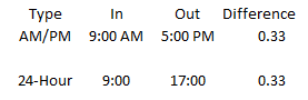
If you’re using the 24-hour clock then it looks okay. However, the calculations are still reading in the time format and while that may work okay for the 24-hour clock, it’s going to cause an issue for the AM/PM. So let’s change the format using the comma style so it doesn’t read like a date. Then, the data looks as follows:

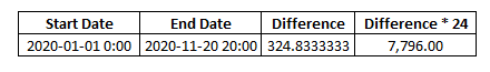
This might seem even more confusing until you realize what Excel is doing. It’s assigning a value between 0 and 1 for the time of day. The value of 0.33 indicates that the time is one-third of the day, which is what an eight-hour shift would be since 8/24 is the same as 1/3.

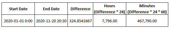
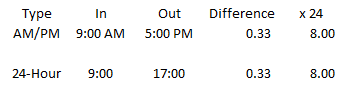
However, using 0.33 isn’t going to be too helpful if you need hours to be able to track how much someone should earn for that shift. To solve this, simply multiply the time difference by 24. Then, your time difference looks as follows:

calculating time difference for am pm and 24-hour time and converting into hours.

Now you see the eight hours that you may have first expected to see when calculating the difference between these times. Since it’s now reading as a number, you can multiply this by an hourly rate and arrive at the pay that is owing for the shift.

If you’re not looking for hours and just want the total minutes, then all you need to do is just multiply by a factor of 60 to convert the eight hours into 480 minutes.

Calculating hours worked when someone works the night shift

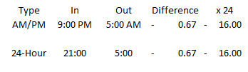
The above calculations work well if someone is working within the same day, but if someone starts at 9:00 PM and ends at 5:00 AM the next day, it’s not going to calculate properly if you simply take the difference between the numbers. In fact, the number would come out negative:

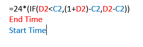
That’s obviously not what you’ll want. To account for this, you’ll need to add an IF statement into our formula. The IF function should look at whether the end time is earlier than the start time. If it is, you’ll want to add 1 to the calculation. Here’s how the formula for the difference calculation would look like:

adjusting time calculations for overnight shifts.

I include the 24 in the calculation so that I don’t need to use an extra cell to convert the difference into hours. All the formula is doing is looking at if the end time is before the start time, and if it is, add a 1 to the end time before subtracting the start time from it. This method will work whether you’re using a 24-hour clock or the AM/PM format:

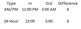
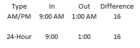
This method will work even if someone works a 16-hour shift:

Knowing how to calculate time difference in Excel isn’t difficult, and the key points to remember are as follows:

Ensure the time is entered correctly, and
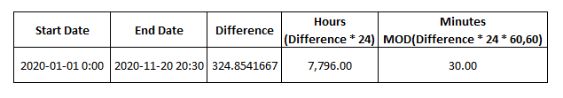
Multiply the difference between the times by a factor of 24 for hours and another factor of 60 if you only want minutes.

Calculating time difference in Excel when the data is in text

If you need to know how to calculate time difference in Excel and you don’t have the luxury of the data being in the right format, the good news is it’s still possible to do so.

For instance, what if you want to enter the entire start and end times within one cell. In that case, you’re always going to be running into this situation. Suppose someone enters the following value into a cell: 9:00 AM-5:00 PM.

The format would be correct if there weren’t multiple times in that cell, which ensures it will read as text. That’s where you’ll need to use some data manipulation that involves using the MID function.

Let’s start by pulling the start time. For this, we’ll grab the numbers that come before “AM” but because it doesn’t matter whether it’s AM or PM, we’ll search for the letter “M” on its own:

=MID(A1,1,FIND(“M”,A1,1))

Here’s a breakdown of the formula:

Argument 1: A1 is the cell we’re looking at.
Argument 2: Start pulling from the first character.
Argument 3: The length of the text goes up until the letter “M” is found.

The formula will yield a result of 9:00 AM. However, you’ll still need to convert this into a number and you can do this by multiplying the result by 1 or putting it inside the TIMEVALUE formula:

=TIMEVALUE(MID(A1,1,FIND(“M”,A1,1)))

This will now give us a value of 0.375 and it can be used for the calculation. Next up, we’ll calculate the ending time. To do this, we’ll again use the MID function but the key is to start pulling the data after the dash (-) sign:

=MID(A1,FIND(“-“,A1,1)+1,LEN(A1))

This one is a bit more complicated, but let’s look at the different arguments again:

Argument 1: Still looking at cell A1.
Argument 2: Use the FIND function to get to the position where the dash (-) is at and then add a 1 onto that to ensure we’re starting from where the number begins and not the dash (-).
Argument 3: Even though you don’t need the total length of the string, you can use the LEN function to ensure the formula get everything that comes after the dash (-).

Doing this will give us a result of 5:00 PM and by again adding the TIMEVALUE function into it, it will give us a result of 0.7083

=TIMEVALUE(MID(A1,FIND(“-“,A1,1)+1,LEN(A1)))

You can now combine these formulas into one to do the calculation with text:

=TIMEVALUE(MID(A1,FIND(“-“,A1,1)+1,LEN(A1)))-TIMEVALUE(MID(A1,1,FIND(“M”,A1,1)))

This will result in 0.33 for the time difference, which is the correct result. However, with shifts that stretch into the following day, you’ll again run into the issue of how to deal with calculating time. If you don’t have night shifts to worry about, you can stop here.

But if you need to factor them in, then the easiest way to do so is using the AND and IF functions. We’ll want to look at whether the last two characters end in “AM” while also looking at whether “PM” is in the text:

=IF(AND(RIGHT(A1,2)=”AM”,(NOT(ISERROR(FIND(“PM”,A1,1))))),1,0)

Here’s a breakdown of the formula:

The first formula inside the AND function looks at the last two characters in the text to see if they equal “AM”
The second function looks for the characters “PM” anywhere in the cell. If it’s not found it will result in an error, that is why the formula begins with NOT and ISERRROR; you’ll want to add a 1 if it isn’t causing an error and “PM” is found.
If both of the above conditions are met, a value of 1 will be returned. Otherwise it will result in 0. This can now be added to the earlier time calculation formula, added to the end time.

Here’s how the complete formula will look like after adjusting the end time in case there’s a cross over from PM into AM:

=IF(AND(RIGHT(A1,2)=”AM”,(NOT(ISERROR(FIND(“PM”,A1,1))))),1,0)+TIMEVALUE(MID(A1,FIND(“-“,A1,1)+1,LEN(A1)))-TIMEVALUE(MID(A1,1,FIND(“M”,A1,1)))

It’s a messy formula but it is only adding the 1 to the end time if it’s a PM start time and ends in the AM. The only thing left would be to multiply this all by 24 to get the entire shift total in hours:

=24*(IF(AND(RIGHT(A1,2)=”AM”,(NOT(ISERROR(FIND(“PM”,A1,1))))),1,0)+TIMEVALUE(MID(A1,FIND(“-“,A1,1)+1,LEN(A1)))-TIMEVALUE(MID(A1,1,FIND(“M”,A1,1))))

The key thing to note is for this formula to work it’s important to leave a space between AM and PM. For example, if I were to just enter 9:00AM, Excel wouldn’t read that properly and it would result in an error. By leaving a space, it helps with parsing the data out, otherwise the formula would need to be even more complex. If it isn’t in that format, it’s preferable to first clean up the data as opposed to building a very complicated, nested formula using IFs and MIDs.

The above example goes over a few scenarios and obviously you can adjust the MID and other functions as needed based on how your inputs look. Pulling date calculations out from text is possible, it’s just no very pretty.

If you liked this post on how to calculate time difference in Excel, please give this site a like on Facebook and also be sure to check out some of the many templates that we have available for download. You can also follow us on Twitter and YouTube.

Calculating Date Differences Using VBA

February 26, 2017

by admin with No Comment dates functions vba

In VBA there is a custom DateDiff function that allows you to easily calculate the difference between dates – whether you want the difference to be in days, weeks, months, years, it is easier to accomplish this in VBA than through regular Excel formulas. I have piggy-backed off the DateDiff function to make a custom function in Excel that makes it easy to use as a formula in your spreadsheet.

The custom function I have created is called datecalculation and consists of three arguments: start date, end date, and interval. The interval determines how the difference is calculated. The interval needs to be in quotations and use one of the following codes:

Below is an example of how the function work when computing the difference between January 1, 2016 (cell C2) and January 1, 2017 (cell C3). The interval codes are in column A.The result column is the date difference according to the selected interval.

To make this function work in your spreadsheet simply insert the following VBA code. If you are not sure how to do that, please refer to this post, specifically the section about inserting VBA code.

————————————————————————————————————————

Function datecalculation(date1 As Date, date2 As Date, interval As String)

datecalculation = DateDiff(interval, date1, date2)

End Function

————————————————————————————————————————

Incrementing dates by month using a formula vs autofill.

How to Do Date Calculations in Excel (and Format Them)

February 19, 2017

by admin with 3 Comments dates intermediate

In this post, I am going to cover some commonly used date functions and show you how to do some basic date calculations in Excel.

Incrementing Dates by Days and Months

One of the more common date calculations in Excel is to increment your dates. If you want to increment a date by months, years, or days, then you can use the DATE function to do so. This function has three arguments: year, month, and date. If I have a date in cell C3 and I want to make cell C4 one month later, I would use the following formula:

=DATE(YEAR(C3),MONTH(C3)+1,DAY(C3))

For each of the year, month, and day arguments I used their individual functions. The YEAR function will take the year of the date specified, as the MONTH function will take the month, and the DAY function will take the specific day. For the DAY and YEAR functions I simply just referenced cell C3 since I want those values to remain the same. The MONTH function also took the same value from cell C3, however, I added +1 to it as well to increment the value by one month.

If I want to just increment by day, then I can just enter a starting date and drag that value down, and Excel’s autofill will automatically increment the values by one day. Here’s a comparison of the daily increment (where no formula is necessary) and the monthly increment, where I use the formula noted above:

Now, there is another way, an even simpler way, just by using Excel’s autofill feature that I can increment by month. If I enter my starting date in cell B3 and pull it down using the fill handle, Excel will increment by day. However, if I select cell B3 and pull down the fill handle while also holding down the right-click button, it gives me the option to select how I want to increment – including fill days, weekdays, months, and years.

This way you can ensure Excel increments as you like. If you just use the fill handle without the right-click button you don’t get these options and Excel fills in the data how it thinks makes sense. Interesting to note that if you fill in cell B4 with the next month, and then select cells B3:B4 and then use the fill handle, then Excel has figured out you want to increment by months and doesn’t increment by days anymore. The more of a pattern you show Excel, the more likely it will know what you are trying to do.

In the above picture if I now double click the fill handle my daily increment will become monthly since I have selected two points in my series. And since the two points have a monthly interval, Excel assumes I want the rest of the series to also have monthly intervals as well. The result becomes this:

You may wonder what the point would be of using the date function in the formula above if you can just use the fill handle since it is faster and easier. The main benefit of using a formula is if you don’t want to have to use the fill handle all the time. If you just need to set up your dates one time, then certainly the fill handle makes sense. But if you are working with a large data set that you will continually add to, you might find it a bit easier to have a formula there as opposed to using the fill handle each time and making sure it is incrementing correctly.

Calculating the Difference From/To Today

If you want to include today’s date in your calculations, you can use the TODAY() or NOW()functions. These functions have no arguments and you just enter them with both parentheses. This will generate today’s date. The difference between the two functions is the NOW() function also includes the time. But for the purpose of calculating the difference in days, either one will do the job.

NOW() and TODAY() Functions

Alternatively, you can use the shortcut CTRL+; which will plug in today’s date. If you want the date to update every time you open the spreadsheet then you are better off using the functions. If you want to do a one-time insertion of the current date never to change later, then the shortcut will do. It is no different than just entering the date yourself.

End of Month Calculations

Suppose I wanted to not calculate the number of days from today, but the end of the month. What I could use is the EOMONTH function. This has two arguments – start date, and months. If I wanted to use the end of the current month, I would enter the following formula:

=EOMONTH(TODAY(),0)

If I wanted the end of next month, then I would change the 0 to a 1:

=EOMONTH(TODAY(),1)

The months argument just tells Excel how many months ahead to go. Whether you change the months argument or alter the start date to get to a later month end value, it doesn’t matter, both methods can get you to the desired result.

EOMONTH Function

Calculating Workdays

Up until now, I’ve gone over how to calculate the difference in days. But suppose I wanted to calculate only working days. To do this you can use the NETWORKDAYS function which will take the starting date, ending date, and calculate how many workdays fall in between. To be more accurate you could also include a list of holidays into the function (which you will have to populate).

NETWORKDAYS Function

In the above example, I selected Jan 2 and 3rd as holidays so as a result, the NETWORKDAYS function with holidays has two days fewer than the function without holidays since those days both fall within the date range. Without a list of holidays, the NETWORKDAYS function effectively calculates weekdays since it would only ignore weekends. Also note that in the argument for holidays, do not include any text fields such as a header for holidays. If my range included the header then it would return a #VALUE error.

A similar function, WORKDAY takes the starting date, and you select how many workdays you want to advance by, and it will return a date result for the next working day after the days you specified. Again, you can list the holidays to ensure a more accurate calculation.

WORKDAY Function

If you don’t use holidays then both functions (NETWORKDAYS and WORKDAY) will not adjust for them. However, both functions will recognize and skip over weekends and so if you leave holidays blank they effectively just look at every weekday.

Calculating Weeks, Months, Years

If I wanted to do date calculations in Excel to show the difference between two dates in weeks, what I could do is use the WEEKNUM function and then use my date as the argument for that function. Once I calculate this for both dates then I just calculate the difference. This strictly looks at the week of the year, so it won’t take into account whether one date is a Friday and the other a Monday.

WEEKNUM Function

And if you wanted to you would be better off dividing the difference in dates by 7 to get fractional weeks.

For months you can do the same thing, except using the MONTH function which will yield a result from 1 to 12. The YEAR function will do the same as the month function, give you the year of the specified date, which you then can use in your calculations to calculate the change in years. You can also use the YEARFRAC function if you wanted to calculate the difference in fractions of a year, to give you a more specific result when calculating the difference in years.

YEARFRAC Function

Formatting Dates

In addition to just doing date calculations in Excel, it’s important that your dates are also formatted properly. You can format dates so they display exactly how you like right through the format cells option. The easiest way to do that is to go to the cell formatting (right-click format cells, or click ctrl+1), and select the CUSTOM category.

Custom Date Formatting

If you want month/day/year (which it may already be set to) the formatting is just m/d/yyyy. But what if I didn’t want to show all four numbers for the year, just the last two? Then I would set it to m/d/yy. You can flip the d and the m around so it is d/m instead of m/d and then you have day/month/year. If you use two d’s rather than one you will get a 0 if you are in single digits for the day. For instance, instead of 1/1, you could get 01/01. You will notice the changes in the sample box above as you change your custom category.

Here is a quick summary of the use of letters and what results they will yield:

m or d: will use 1, 2, 3, etc.
dd or mm: will use 01, 02, 03, etc.
ddd or mmm: will spell out the abbreviation (e.g. ‘Mon’ for Monday, or ‘Nov’ for November)
dddd or mmmm: will spell out the entire day or month (e.g. Monday, November)
y or yy: will use the last two digits of the year.
yyy or anything more: will use the full four digits of the year.

If I wanted to use a formal date that showed the day and month spelled out, followed by the numerical day, a comma, and the year, I would use the following format:

dddd mmmm d, yyy

Date Format

If you liked this post on How to Do Date Calculations in Excel (and Format Them), please give this site a like on Facebook and also be sure to check out some of the many templates that we have available for download. You can also follow us on Twitter and YouTube.

Formula to find day of week occurrences in Excel

April 26, 2014

by admin with No Comment advanced dates

In my previous post I showed a function that can help pull a certain instance of a day of the week using VBA. In this post, I’ll show how to do that without VBA. Specifically, three things this post will look at: 1) how to find the first Monday of the month 2) how to find the date ending/starting of a week, and 3) how to find the 3rd Monday of the month

1.Finding the first Monday of the month

First, I need to identify the weekday that the first day of the year falls on with this formula:

Formula 1.A

=WEEKDAY(DATE(2014,1,1))

This returns 4 (Wednesday).

Next I’ll determine how many days away this is from my desired day – Monday. Since Monday is the 2nd day of the week, the first day of the year is 2 (4-2) days after Monday. If you want to use another day instead of Monday then change the 2 to the corresponding day of the week (for example, Sunday is 1 – assuming your settings are setup for weeks starting on a Sunday).

With 7 days in a week, I need to deduct 2 from 7, making 5 days that I need to add to the first day of the year to get to the first Monday of the year. The formula so far looks like this:

Formula 1.B

=DATE(2014,1,1)+7-(WEEKDAY(DATE(2014,1,1))-2)

However, this formula will only work if the first day of the month falls after Monday. I need to include an IF statement so that in the case that Monday (or whatever day I choose) falls after the first day of the year, it will just add the difference. The formula that follows includes this consideration:

Formula 1.C

=DATE(2014,1,1)+IF(WEEKDAY(DATE(2014,1,1))-2<=0,2-WEEKDAY(DATE(2014,1,1)),7-((WEEKDAY(DATE(2014,1,1))-2)))

(the numbers highlighted in red relate to the day of the week I want to calculate)

This formula is a bit more complex but all it is saying is that if the difference between the days of the week are negative (e.g. first day of the year is Sunday and hence before Monday) then I would just add the difference to the first day of the month. Otherwise the formula remains as it was.

I’ve replaced all the possible variables with words so you can easily see where to change the values to calculate to the day you want.

Formula 1.D

=DATE(YEAR,MONTH,1)+IF(WEEKDAY(DATE(YEAR,MONTH,1))-WEEKDAYNUMBER<=0,WEEKDAYNUMBER-WEEKDAY(DATE(YEAR,MONTH,1)),7-((WEEKDAY(DATE(YEAR,MONTH,1))-WEEKDAYNUMBER)))

2. How to find the 3rd Monday of the month

Continuing from Formula 1.D, I’m going to make an adjustment to calculate the proper week. To do this I need to add two weeks to the formula:

Formula 2.A

=DATE(YEAR,MONTH,1)+((XTHOCCURRENCE-1)*7)+IF(WEEKDAY(DATE(YEAR,MONTH,1))-WEEKDAYNUMBER<=0,WEEKDAYNUMBER-WEEKDAY(DATE(YEAR,MONTH,1)),7-((WEEKDAY(DATE(YEAR,MONTH,1))-WEEKDAYNUMBER)))

Where XTHOCCURRENCE in this case will be equal to 3.

If your result is a number you will need to change the cell format (CTRL+1) to date.

3. Find the date ending/starting of a week

If you have weekly reporting and reference a week number, you may find it useful to show what date that week relates to.

This formula builds off of Formula 1.D. One difference is the month will always be set to 1 because we need to know the first weekday of the year. This is important to determine the number of weeks that need to be added.

If the first day of the year falls after the day I want (this example is Monday), then I know the first Monday will fall in week 2, not in week 1. What that means is if I want to determine the Monday on week 15, I will need to multiply by 13 and not by 14 weeks to get to that date. The formula is:

Formula 3.A

=DATE(2014,1,1)+IF(WEEKDAY(DATE(2014,1,1))-2<=0,(15-1)*7+2-WEEKDAY(DATE(2014,1,1)),(15-2)*7+7-((WEEKDAY(DATE(2014,1,1))-2)))

The only parts I added were those in purple, which just multiply the number of weeks I need. This formula will work for any day of the week. So if you want to calculate the the start or end of week 15, you can set the weekday you are calculating to as Monday (2) or for the end of the week to Friday (6). Here is the formula with the variables replaced with words:

=DATE(YEAR,1,1)+IF(WEEKDAY(DATE(YEAR,1,1))-WEEKDAYNUMBER<=0,(WEEKNUMBER-1)*7+WEEKDAYNUMBER-WEEKDAY(DATE(YEAR,1,1)),(WEEKNUMBER-2)*7+7-((WEEKDAY(DATE(YEAR,1,1))-WEEKDAYNUMBER)))

The weekday number relates to the day of the week (e.g. 1-Sunday, 2-Monday, 3-Tuesday, 4-Wednesday, 5-Thursday, 6-Friday, 7-Sunday). This may be slightly different depending on your regional settings, you may have Monday set as 1. The weekday number is the day of the week that you’re interested in determining where it falls.

Find the xth occurrence of a day in a month

April 19, 2014

by admin with No Comment advanced dates functions vba

This function is called dayx. It consists of the following arguments: occurrence number, day of the week, month, year. For example:

dayx(2,”Monday”,10,2014) or dayx(2,1,10,2014) will return the second Monday of October 2014, which is October 13, 2014

For information on how to insert a custom function, see this post.

Here is the code for this function:
———————————————————————————————————————–

Function dayx(xoccurrence As Long, xday As String, xmonth As Long, xyear As Long)

Dim firstweekdayofmonth As Long
Dim currentmonth, endofmonth, firstdayofmonth As String

Select Case UCase(xday)
    Case Is = “MONDAY”
        xday = 1
    Case Is = “TUESDAY”
        xday = 2
    Case Is = “WEDNESDAY”
        xday = 3
    Case Is = “THURSDAY”
        xday = 4
    Case Is = “FRIDAY”
        xday = 5
    Case Is = “SATURDAY”
        xday = 6
    Case Is = “SUNDAY”
        xday = 7
End Select

‘Convert month number to name
currentmonth = Format(DateAdd(“m”, Val(xmonth) – 1, “January 1”), “mmmm”)
endofmonth = Format(WorksheetFunction.EoMonth(Format(DateAdd(“m”, Val(xmonth) – 1, “January 1”), “mmm dd, yyyy”), 0), “mmmm dd, yyyy”)

‘Determine the first day of the month
firstdayofmonth = Weekday(currentmonth & ” 1, ” & xyear, vbMonday)

‘Calculate
If xday >= firstdayofmonth Then
dayx = Format(currentmonth & ” ” & (7 * (xoccurrence – 1)) + 1 – (firstdayofmonth – xday) & ” , ” & xyear, “mmmm d, yyyy”, vbMonday)
Else
dayx = Format(currentmonth & ” ” & 7 + (7 * (xoccurrence – 1)) + 1 – (firstdayofmonth – xday) & ” , ” & xyear, “mmmm d, yyyy”, vbMonday)
End If

dayx = Format(DateAdd(“m”, 0, dayx), “mmmm dd, yyyy”)

End Function

———————————————————————————————————————–