How to Calculate Internal Rate of Return (IRR) in Excel

Last week, I covered how to calculate discounted cash flow. In this post, I’ll build off that worksheet and show you how you can calculate the internal rate of return (IRR) in Excel. IRR tells you the return that you’re making on an investment or project, and at what discount rate the net present value of all the cash flows will be zero. In these scenarios, there’s typically an outlay of cash, usually at the beginning.

In my previous example, I only looked at cash flows coming in. This time, I’ll look at a scenario where you pay money out at the beginning and generate cash flow in future periods. A common example is paying to upgrade a piece of equipment and then generating cost savings from it for x number of years. Knowing the IRR can tell you if you’re making enough of a return off of the investment and whether you should move forward with it. Using IRR can also be helpful when you’re comparing multiple options to see which one is the best one.

Setting up the spreadsheet

This step is about the same as when setting up the discounted cash flow template. You’ll need to enter the different years, the cash you expect to come in or out, and then calculate back what the present value is today.

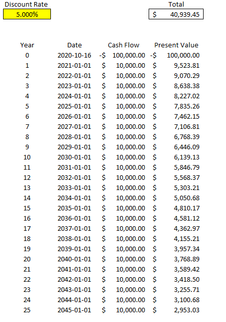
Here’s what the file looks like setting in a scenario where you pay $100,000 upfront and then generate $10,000 in cash flow for 25 years. At a 5% discount rate, in this example the present value of all that cash flow is a positive $40,939.45:

Calculating the IRR

The problem here is the discount rate can be difficult to determine, and that can have a significant impact on your overall returns. And so rather than worry about what your discount rate should be, you only need to determine the IRR — which is to say at what point would your present value be worth $0? If you need a higher return than the IRR the project would be a no-go but if you’re okay with anything up to and including the IRR, then the project or investment would be passable. What it comes down to is the lower the IRR is, the worse the investment is

There are a couple of different ways to calculate IRR in Excel. One way is through a formula called XIRR. It only has two required arguments — dates and cash flow. This is why in this example I entered dates for my cash flows rather than just numbering the years. This makes it easier for me to use the XIRR formula. In my spreadsheet, I enter the following formula:

=XIRR(D6:D31,C6:C31)

Column D contains my cash flow and column C contains the dates. Doing this, Excel tells me the IRR is 9.687% for this specific project. But if I work backwards and calculate the net present value, it doesn’t get me right to 0:

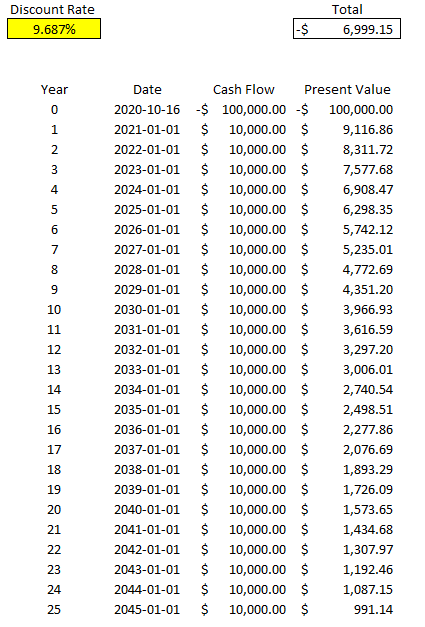
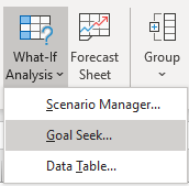
It certainly gets close to 0 and it’s probably close enough that it can help you make a decision about your investment. However, there’s another way to calculate IRR and that’s using Excel’s What-If Analysis. On the Data tab, there’s a drop-down for this option in the Forecast section:

Depending on which version of Excel you’re using, it may show a bit differently, but what you’re ultimately looking for is Goal Seek.

Goal Seek is an accelerated way of doing trial-and-error. Excel’s doing it for you much quicker than you could ever do it by yourself. For IRR, it’s the best solution.

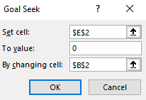
Here’s how it works. You’ll need to enter the cell that you want to get to a certain value, what value that is, and which cell Excel should be changing values in. In my spreadsheet, E2 is where my net present value formula is, and I want that to equal 0. In cell B2 is my discount rate, which is what I want Excel to be changing. Here are what my inputs look like:

Then, once I click on OK, Excel goes to work. After a few seconds you should see Excel show you that the target value and the current value are a match (e.g. they’re both 0), meaning it’s done its job successfully:

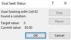
Now, if I look at my template, I see a different discount rate and my total present value is netting out to 0:

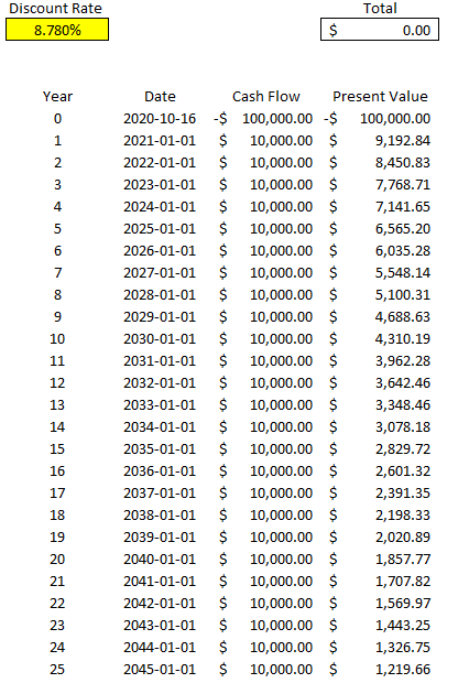
As you can see, this is much more accurate than Excel’s XIRR function. You can repeat these steps and make this table for other projects that you can assess side-by-side.

If you’d like to test this out, try downloading the discounted cash flow spreadsheet from my last post and then just using Goal Seek or the XIRR function to determine your IRR. You can remove unnecessary columns from the sheet and then duplicate the table, and then you’ve got a template where you can assess multiple investments against one another.

If you liked this post on how to calculate IRR in Excel, please give this site a like on Facebook and also be sure to check out some of the many templates that we have available for download. You can also follow us on Twitter and YouTube.