How to Pull Foreign Exchange Rates Into Excel Using Power Query

In a previous post, I showed how to get stock prices using Power Query. This time around, I’m going to show you how we can do the same for foreign exchange rates, pulling that data into Excel. For this example, I am going to use the currency conversion site xe.com.

Creating the connection

The first thing that we need to do when creating a Power Query connection is determining which web page the data will come from. On the xe.com website, there is a currency table for each day. If I wanted to pull the USD foreign exchange rates into Excel as of August 22, the URL I would use is as follows:

https://www.xe.com/currencytables/?from=USD&date=2021-08-22

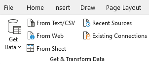
The link is convenient because I can easily alter the currency and the date. I’ll go over how to do that later but first, let’s create the connection. To do that, go in the Data tab on the Ribbon and click on From Web button under the Get & Transform Data section:

Then, on the next screen, I’ll paste the link and click OK:

Once it has loaded, there will be multiple tables to choose from. Table 0 is the one that has the exchange rates:

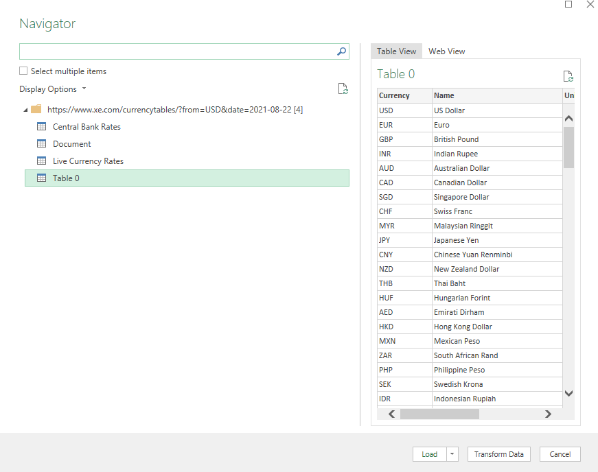
Instead of clicking to load the data, click on Transform Data to make any adjustments to it before it loads into Excel.

Adjusting the query

Once the query is loaded, you’ll see the following window:

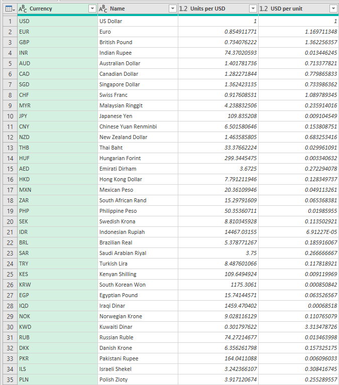
You probably don’t need or want to see all these rows in Excel. So what you can do before loading it is to clean the data up a bit. Let’s say I only want to pull the US exchange rates in Excel for EUR, GBP, CAD, and AUD. To do that, I’ll click on the Currency header and filter for just those options. You can filter the same way you would an Excel table. And once you’re done, you should see the table get a whole lot smaller:

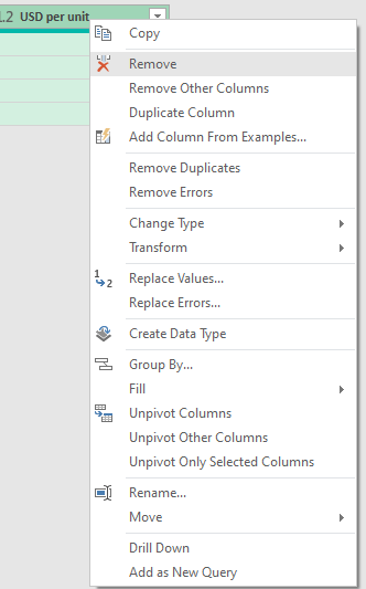
To cut down the table even more, I can remove the Name field since. To remove any column, simply right-click on it and click Remove:

Clicking on the Load & Close button will now populate this into my Excel sheet:

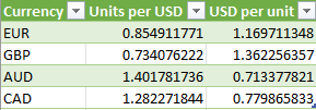
Now, let’s alter the URL so that it can be adjusted dynamically for both the currency and date.

Using variables in the Power Query link

An advantage of using a link that has the currency and the date in it is that it is easy to change. I’m going to start by creating a couple of variables. The first is for the currency, and the second is the date. I’ve set up named ranges of ‘Currency’ and ‘Date’ the following fields:

When entering the date, I’m entering an apostrophe (‘) first so that formatting isn’t an issue and Excel reads the value as text.

What I’m going to do next is go into Power Query and create these variables. To do so, go back into the Data tab and click on Queries & Connections. Off to the right, you should see your query. Right-click on it and select Edit:

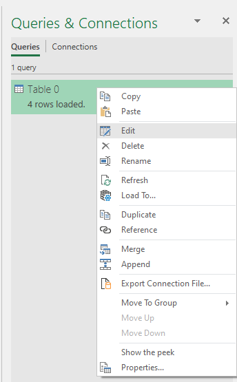
This will open Power Query back up. I’m going to click on Advanced Editor button on the Ribbon, under the Query section:

At the top of the code, I’m going to insert two lines. One for each variable:

Currency = Excel.CurrentWorkbook(){[Name=”currency”]}[Content]{0}[Column1]

Date = Excel.CurrentWorkbook(){[Name=”date”]}[Content]{0}[Column1]

I will also need to adjust the Source, so that instead of this:

Source = Web.Page(Web.Contents(“https://www.xe.com/currencytables/?from=USD&date=2021-08-22”))

It becomes this:

Source = Web.Page(Web.Contents(“https://www.xe.com/currencytables/?from=”&currency&”&date=”&date))

The variables are ready to go. But before using these them, it’s important to remove the Changed Type step from Power Query:

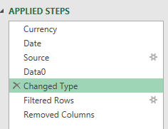
This step looks for exact column names which can cause an error if your names change when downloading data.

Now with that done, you can change the values and your table will change. Here’s what it looks like if I change the currency to AUD and set the date to July 31:

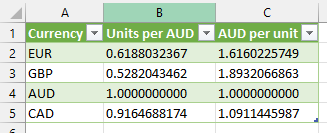
The one problem, however, is that now I have AUD and don’t have USD. What I can do is create a separate table of all the currencies I want to pull in:

I can load this table into Power Query by going back into the Data tab and this time clicking on the From Sheet option. I’ll rename the FXtable and it shows below the other table:

Now, if I only want to see the values from FXtable, what I will need to do is merge the queries.

Merging queries in Power Query

Switch over the Table 0 query and get rid of the Filtered Rows step. Then, on the Home tab, there is an option to Merge Queries in the Combine section that you’ll want to click:

On the next screen, I’ll select the FXtable from the drop down and select the currency fields from each table:

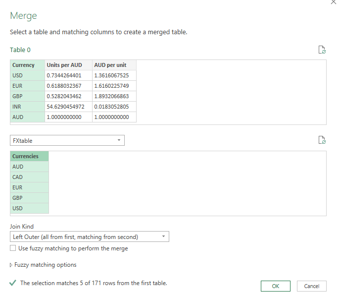
Leave the default of Left Outer selected and then click OK:

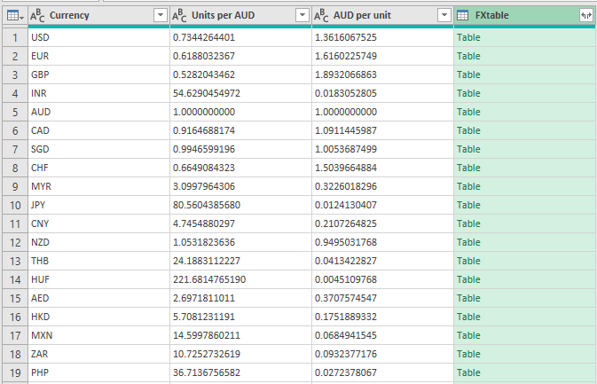
Next, click on the button on the FXtable to expand the table:

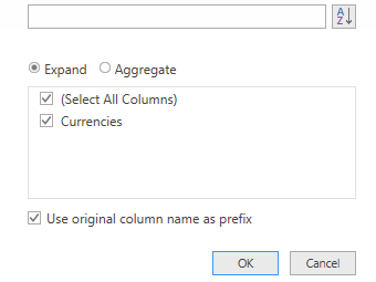
Click OK on the next section to expand the only field from that table:

Which will result in this:

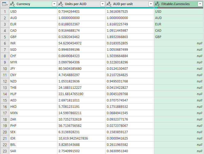
Then, just filter the FXtable.Currencies field so that null values don’t show up, and you’re left with just the currencies that were present on that table:

Now that the table has served its purpose, I can remove the FXtable.Currencies column and I’m back to what I had before:

Now, I can modify the base currency, the date, plus the currencies that I want to show up. Suppose I just want to see the EUR-GBP currency rates for Jan 1, I could enter the following values:

All you need to do is refresh the data from the Data tab and all the queries will update:

And the data matches what comes from the xe.com site:

Are you looking for a way to pull historical data for a currency pair? You can use Yahoo Finance to do that, and the steps for doing that query is similar to how you would pull stock quotes from there (refer to the link at the top of this post).

If you liked this post on How to Pull Foreign Exchange Rates Into Excel Using Power Query, please give this site a like on Facebook and also be sure to check out some of the many templates that we have available for download. You can also follow us on Twitter and YouTube.