

Excel is a great program for data analysis. And one of the key tools that analysts can use within it is Power Query. While it can seem intimidating for novice users, this guide will walk you through how to use it and how it can help you analyze data.
Getting started with Power Query
Power Query is an Excel tool that enables users to connect, combine, and refine data sources easily. It’s especially useful for automating the data cleaning and preparation process. With Power Query, repetitive tasks like importing data, filtering, sorting, and other transformations become streamlined, saving valuable time.
Power Query was first introduced as an add-in for Excel in 2010 and 2013. However, it became a built-in feature starting from Excel 2016. In these later versions, it’s integrated into the Data tab in the Excel ribbon, offering a more seamless experience compared to the add-in version for earlier Excel releases. Users of Excel 2010 and 2013 can still access Power Query, but they need to download and install the add-in separately. In Microsoft 365 (formerly known as Office 365), Power Query is fully integrated into Excel.
How do I launch Power Query?
To launch Power Query and get started with it, you’ll first want a table or data set in mind that you want to work on. You could link to an external website, workbook, or just have a table or data set within your worksheet that you want to work on. Power Query, after all, is a tool for data analysis — you need data to start with. Here are some of the more common ways to launch Power Query:
1. Connecting to an External Workbook
- Navigate to the Data Tab: Go to the Data tab in the Excel ribbon.
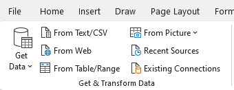
- Get Data: Click on Get Data in the Get & Transform Data section.
- Choose the Source: Select From File and then choose From Workbook.
- Select the Workbook: Browse and select the external Excel workbook you want to connect to.
- Load or Transform: Once you select the file, you can choose to either load the data directly into Excel or open the Power Query Editor to transform the data before loading.
2. Connecting to a Webpage
- Navigate to the Data Tab: Go to the Data tab.
- Get Data: Click on “Get Data” in the Get & Transform Data section.
- Select Web as Source: Choose From Other Sources and then select From Web.
- Enter the URL: Enter the URL of the webpage you want to import data from.
- Load or Transform: After connecting to the webpage, you can choose to load the data directly or use the Power Query Editor for transformations.
3. Using a Range or Table Within the Existing Sheet
- Create or Select a Range or Table: You don’t need to have your data formatted in a table for Power Query to load it, however, Excel will convert it to a table once you launch Power Query.
- Navigate to the Data Tab: Go to the Data tab.
- Get Data: Click on Get Data in the Get & Transform Data section.
- Choose From Table/Range: Select From Table/Range.
- Power Query Editor: This will open the Power Query Editor with the selected table data, ready for transformation.
Each of these methods serves a different purpose. Connecting to an external workbook is useful for consolidating or analyzing data spread across multiple Excel files. Connecting to a webpage allows for the import and analysis of data published online, such as tables on web pages. Using a table within the existing sheet is handy for quickly transforming or analyzing data already present in your workbook. In all cases, Power Query provides a robust set of tools for manipulating the data before loading it back into Excel for further use.
What can Power Query do?
Power Query can help adjust your data before loading it into Excel. Here are some of the key things you can do with it:
- Transform data types
- Handle missing data
- Remove duplicates
- Replace values
- Filter data
- Sort data
- Concatenate columns
- Split columns
- Add conditional columns
- Group and aggregate data
Want to follow along with these examples? Download the sample data set I will use here.
Transform data types
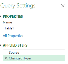
One of the first things Power Query does is it attempts to detect your data types. And when it does, it automatically adjusts them, so that numbers are formatted as numbers, and dates as dates. The Changed Type step appears automatically:
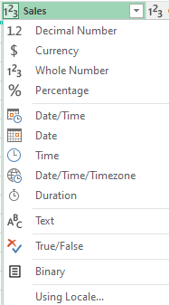
If, however, it hasn’t correctly applied a data type, you can make changes to it. You can specify many different data types, including:
- Text
- Whole Number
- Decimal Number
- Date
- Time
- Date/Time
- Boolean
To change a data type, click on the header which shows the data type that it is, and then you’ll see a list of different options to choose from:
Handle missing data
Power Query in Excel is equipped with a variety of tools to effectively manage missing or null data, a common issue in data analysis. Ensuring accurate handling of missing data is crucial for the integrity of your analysis. Here are the ways Power Query can assist in managing missing data:
- Highlight Null Values: Power Query visually represents null or missing values, making it straightforward to identify gaps in your dataset.
- Remove or Keep Rows with Missing Values: You have the option to filter out rows that contain missing values in one or more columns, useful for analyzing complete records. Alternatively, you might want to focus specifically on rows with missing data.
- Replace Nulls with Specific Values: Power Query allows for the replacement of missing values with a specified value, such as zero, a specific text string, or an average value. This is beneficial where a missing value has a logical default or substitute.
- Fill Down or Up: Filling missing values with the value from the row above or below is possible, which is helpful in datasets where the missing value logically mirrors its neighbor.
- Conditional Replacements: Implement logic to replace or handle missing values based on certain conditions, catering to different scenarios for different categories or columns.
- Aggregate Functions: When performing functions like sums or averages, Power Query automatically accounts for null values, ensuring they don’t skew the results.
- Merging with Missing Data: While merging tables, Power Query can be set up to handle missing values in key columns in various ways, such as including or excluding unmatched rows.
- Data Type Impact: Changing data types might create missing values (like when a text can’t be converted to a number). Power Query helps in identifying and handling such cases effectively.
Removing duplicates
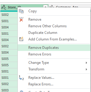
Removing duplicate values is an important part of the cleanup process when it comes to data analysis. If, for example, you’re working with a list of transactions or customer records, removing duplicates ensures that each record or transaction is unique and correctly represented in your analysis. And in Power Query, the process to remove duplicates is a fairly straightforward one. It’s as simple as selecting the column and selecting the option to Remove Duplicates.
You can also apply this for multiple columns at once. To select more than one column, just hold down the CTRL key while clicking on other column headers.
Replacing values
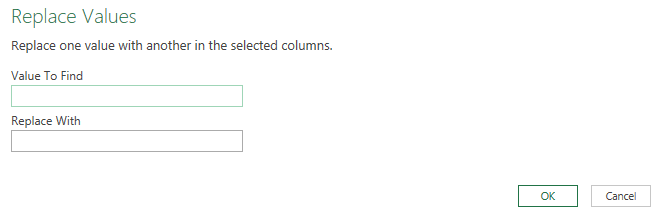
Replacing values in Power Query is a useful feature for cleaning and standardizing your data. It allows you to substitute specific values in your dataset with new ones, which is particularly helpful in correcting errors, standardizing terminology, or handling missing data. Think of it like using the Find and Replace feature in Excel. Here’s how it works:
- Select the column you want to replace values on. Similar to with removing duplicates, you can select multiple columns.
- Select the option to Replace Values.
- In the next dialog box, select the value you want to find and what to replace it with.
Filter data
Filtering data in Power Query is a fundamental aspect of data preparation and analysis, allowing you to narrow down your dataset to only the information relevant for your specific needs. The filtering process is similar to how you would do it in Excel. Here’s how it works:
- Select the column you want to filter.
- Click the drop-down arrow, and you can select how you want to apply your filter:
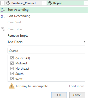
These are the same type of filters you can apply as in Excel, including criteria such as “contains”, “does not contain”, “starts with”, etc. For numeric columns, you can choose from number filters like “equals”, “greater than”, “less than”, and you can specify ranges. For date columns, you can filter by specific dates, before/after a certain date, or choose from a range of date filters.
After setting your filter criteria, Power Query will display only the rows that meet the criteria. You can apply multiple filters across different columns.
Filtering in Power Query is a versatile tool, allowing for basic operations like removing irrelevant rows, as well as more complex data segmentation, which is essential for detailed and accurate data analysis.
Sorting data
Sorting data in Power Query allows you to organize your dataset in a meaningful order, making it easier to analyze and understand. And by doing it in Power Query, when the data is loaded into Excel, your sorting rules have already been applied. Just like with filtering, the process for sorting data in Power Query is also comparable to how you would do it within your spreadsheet:
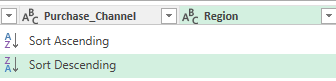
- Choose the column to sort by.
- Select the sort order. For a simple, one-level sort, use the sort ascending (A to Z) or sort descending (Z to A) buttons in the Home tab of the Power Query ribbon. To sort ascending, click the small arrow in the column header and choose “Sort Ascending”. This will organize the data in that column from lowest to highest (e.g., A to Z, 0 to 9, earliest to latest date). To sort descending, click the arrow and choose “Sort Descending”. This will organize the data from highest to lowest (e.g., Z to A, 9 to 0, latest to earliest date).
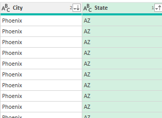
If you want to sort by multiple columns (for example, first by state, then by city), sort the most significant column first, and then sort by the next column. When you apply multiple sorting rules, you will see a number next to the sorting icon to show you its priority. In the screenshot below, the State field has a 1 next to the up arrow, indicating that the data is first sorted in ascending order by state. Then, it sorts the City field in descending order.
Concatenate columns
Concatenating fields (or columns) in Power Query involves combining the contents of two or more columns into a single column. This process is useful for creating unique identifiers, combining textual information, or formatting data in a more useful way. In this example, we’ll combine the State and City fields, by taking the following steps:
- Select the two or more columns you want to concatenate or merge together. The order of your selection is important. If you want the City field first, then that is the one you need to select first.
- Right-click and select the option to Merge Columns
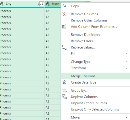
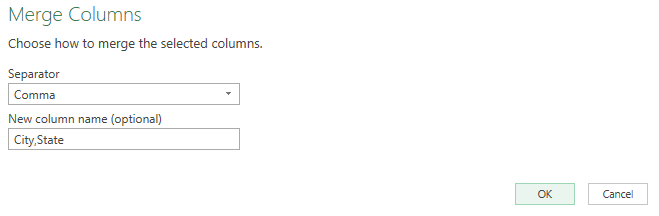
- Specify if you want them to be separated in any way. In this example, we’ll use a comma so that it is in City,State format.
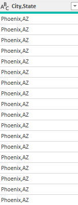
This results in a field that has grouped the two columns. Those two columns have now been replaced with the new merged column.
Split columns
Splitting columns in Power Query is a handy feature that allows you to divide the contents of one column into multiple columns. This can be particularly useful when dealing with data that’s concatenated into a single column but needs to be separated for analysis or reporting. Here’s how we can undo the previous step, to break out the new City,State column back into separate columns:
- Start with selecting the column to split.
- Right-click on the option to Split column. Then select how you want it to be split.
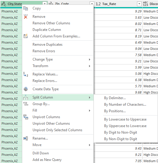
These are the ways you can split them:
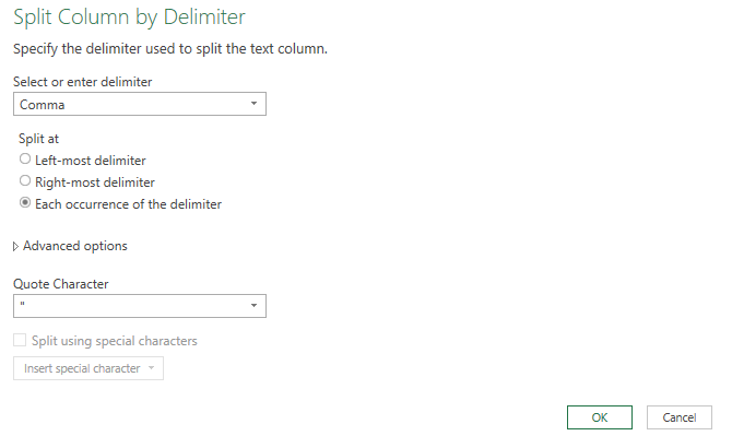
- By Delimiter: Split the column based on a specific character or symbol, such as a comma, space, or custom character. This is the most common method used when data in a column is separated by a consistent symbol.
- By Number of Characters: Split the column into new columns each containing a specific number of characters.
- By Text Length: Split the column at a specific character position.
- Advanced Options: Allow for more complex splits, such as splitting at the first or last occurrence of the delimiter.
In the City,State field, we can split by delimiter — the comma. You can specify how it should be split. But in our example, the default options will suffice:
This will split the columns back into two:
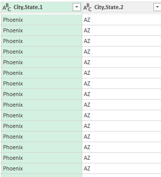
The only thing that may be necessary to do is to rename the columns. To do that, just double-click on the headers and type in a new name for the columns.
Add conditional columns
Adding conditional columns in Power Query is a powerful way to create new columns based on conditions derived from other data in your table. It’s akin to using the IF function in Excel but allows for more complex and multiple conditions. Here’s how you can add a conditional column in Power Query:
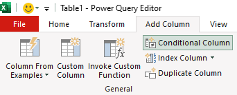
- Select the Add Column tab on the ribbon.
- Select the option to add a Conditional Column.
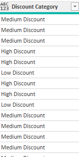
Next, you can create your conditions, and the column name. With the data set in this example, we can set up a column called Discount Category based on the sales price. This can tell us the type of discount a customer is eligible for. The conditions could be as follows:
- If Sales > 3000, then “High Discount”
- If Sales is between 1500 and 3000, then “Medium Discount”
- Else, “Low Discount”
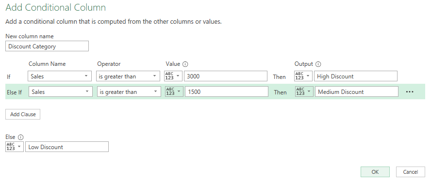
In the above example, the criteria is evaluated in order from top to bottom. This now creates a new column in the table:
Group and aggregate data
Grouping and aggregating data in Power Query is a crucial process in data analysis, allowing you to summarize and analyze large datasets efficiently. This feature is especially useful for finding averages, sums, counts, minimums, and maximums for different categories or groups in your data. In this example, let’s total the sales by city. Here’s how:
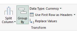
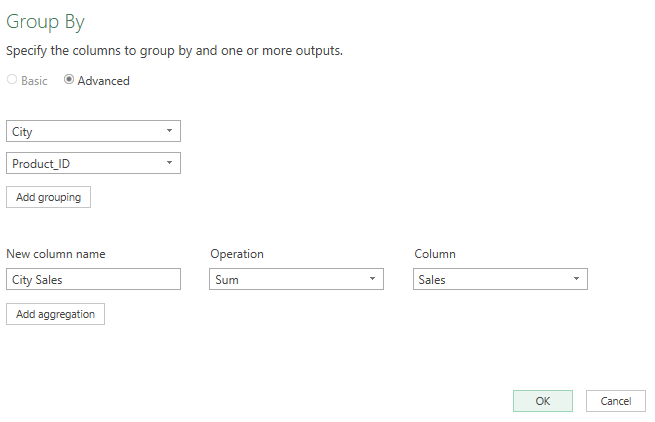
- On the Home tab, click on the Group By button
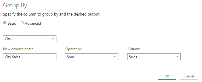
- Select City as the initial field. This is how the data will be grouped.
- Then, enter a column name (City Sales), an operation (Sum), and specify the column to tabulate (Sales)
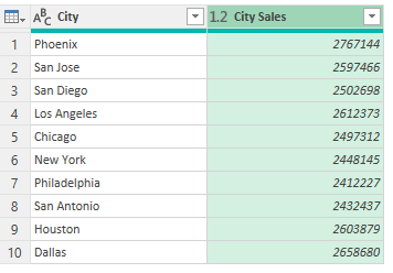
This now gives you a summary by city:
You can also do more complex grouping by more than one field. To do so, select the Advanced radio button when in the Group By dialog box. Then, select Add grouping. In this example, we can add the Product_ID field as another field to group by.
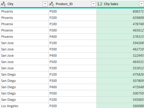
Now, when the grouping is completed, it breaks it down further:
Close & Load once you’re done making changes
Once you’ve finished making your changes in Power Query, you can select the option to Close & Load to get it into Excel.
What “Close & Load” Does:
- Finalizes Changes: When you click “Close & Load”, Power Query applies all the transformations you’ve made to the dataset within the Power Query Editor.
- Loads Data into Excel: After applying the changes, the transformed data is loaded into an Excel worksheet or data model. This can be a new sheet or table, depending on your settings and the nature of your task.
- Creates a Connection: Power Query creates a connection between the source data and the Excel workbook. This connection is maintained, which means that you can refresh the data in Excel to reflect any updates in the source data or further transformations applied in Power Query.
- Saves Transformations: The sequence of steps or transformations you applied in Power Query is saved. This allows for the data to be updated or reloaded with the same transformations applied automatically.
Why it’s beneficial to make changes in Power Query before loading it into your spreadsheet
You may be wondering why you wouldn’t just make all these changes in your spreadsheet. Why is there a need to make the changes in Power Query? Here’s why:
- Data Size Management: Power Query can handle and process large datasets more efficiently than Excel. By filtering, reducing, and transforming data in Power Query, you minimize the load and improve performance in Excel.
- Non-Destructive Data Manipulation: Changes made in Power Query don’t alter the original data source. This means you can experiment with and modify your data without the risk of corrupting the original dataset.
- Automating Repetitive Tasks: Any sequence of steps you apply in Power Query is repeatable. If you regularly receive data in the same format, you can use the same query to process this data, saving time and effort.
- Complex Transformations: Power Query offers more advanced data manipulation capabilities than standard Excel functions, including pivoting/unpivoting, advanced merging and appending, complex filtering, and more.
- Data Cleansing and Preparation: It’s often necessary to clean and format data before analysis. Power Query provides a robust set of tools for handling common data issues like missing values, duplicates, and inconsistent formats.
- Reduces Workbook Size: By transforming data in Power Query and loading only what’s needed, you reduce the overall size of the Excel workbook, leading to better performance and easier handling.
If you like this post on Power Query for Beginners: A Comprehensive Guide, please give this site a like on Facebook and also be sure to check out some of the many templates that we have available for download. You can also follow me on Twitter and YouTube. Also, please consider buying me a coffee if you find my website helpful and would like to support it.