
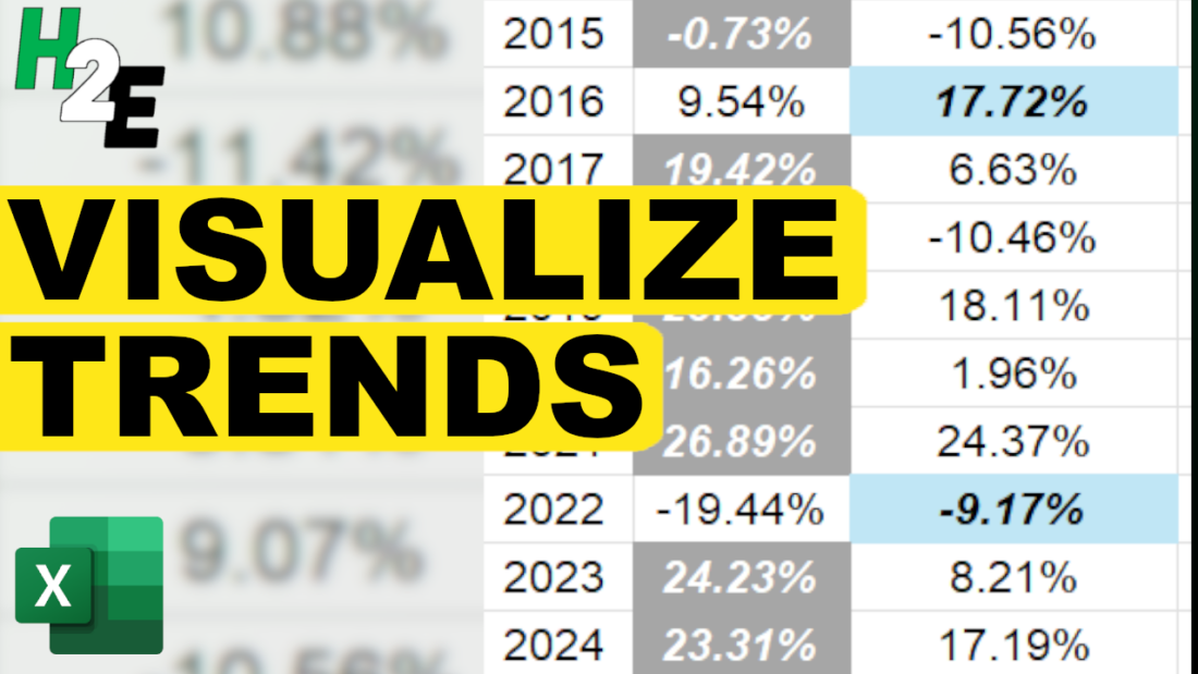
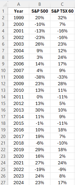
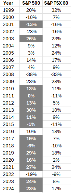
Microsoft Excel can help you analyze data, even without having to do any computations. By simply setting up conditional formatting rules, you can easily visualize data and identify trends. Doing that can help focus your attention on key numbers and make your analysis process much more efficient. In the following data set, I have a list of investment returns by year. I’ll show you how you can setup a rule to highlight which return was larger in each year:
Creating the conditional formatting rule
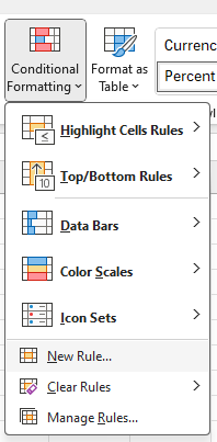
To create a conditional formatting rule to highlight the largest values, I’m going to select column B. Then, I’m going to go into the Conditional Formatting menu on the Home tab and will click on New Rule.
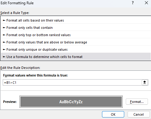
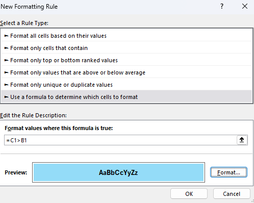
Under the option for the rule type, I’m going to select use a formula to determine which cells to format, and I’ll enter the following formula:
=B1>C1
Then I’ll adjust the format so that the cell has a dark grey color and a white, bolded text.
After clicking apply, the formatting will take effect:
A similar rule needs to be setup for column C. And in this case, I’ll highlight the values in blue.
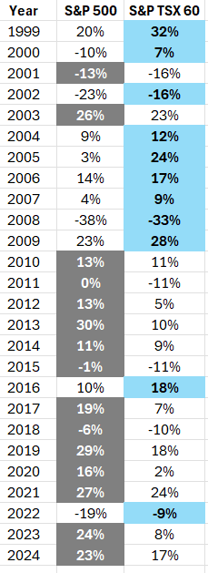
Now there is highlighting applied to both columns:
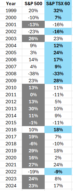
However, the header is also highlighted in column C. To fix this, I’ll add a condition to check to make sure that it is a number:
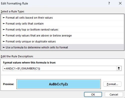
Now the conditional formatting is properly applied, and ignores the header row.
If you like this post on How to Highlight the Largest Values in Excel With Conditional Formatting, please give this site a like on Facebook and also be sure to check out some of the many templates that we have available for download. You can also follow me on Twitter and YouTube. Also, please consider buying me a coffee if you find my website helpful and would like to support it.