Conditional formatting in Excel allows you to automatically format and highlight cells based on their values. You may want to apply custom rules to values that are too high or too low. You may also want to use conditional formatting for budgeting purposes, to show when something is overbudget. Users typically use colors when applying custom formatting. A cell with a high value might be highlighted red versus a lighter color when it is low.
What you can also do is add symbols, including flags, to your conditional formatting rules. This can add another element to make your conditional formatting stand out even more.
Creating conditional formatting rules
In the following example, I have some expense categories, budgeted amounts, actuals, and a field to show when an expense has run overbudget.
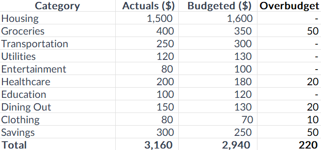
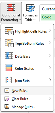
To create conditional formatting rules for this table, you’ll first need to select the cells you want to apply the formatting to. In this case, I’m going to select the Overbudget field and select all the values there. Next, I’ll select the Conditional Formatting button on the Home Screen and click on the option to create a New Rule:
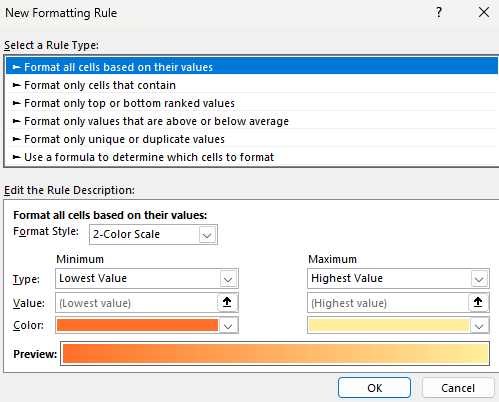
On the next screen, there are many different options for creating rules:
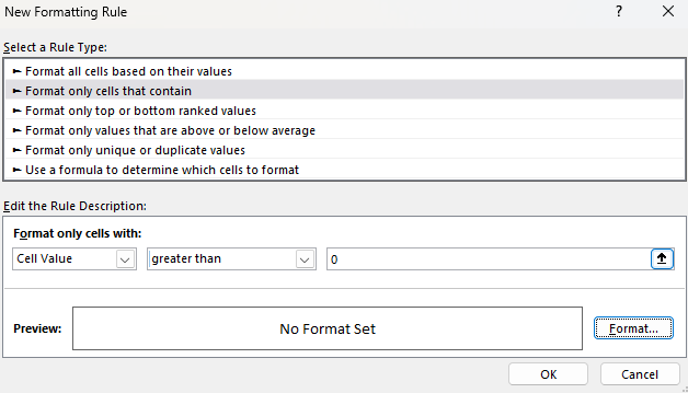
I’m going to select the following option: Format only cells that contain. This allows me to specify a criteria, and then apply formatting to any cells that meet that criteria. Since I’m interested in values that are overbudget, I can create a rule for when the cell value is greater than 0:
Next, I’ll click on the Format button to determine what I want the cells that meet the criteria to look like. If I set the highlighting color to be red and the text to be white, here’s what my table will look like:
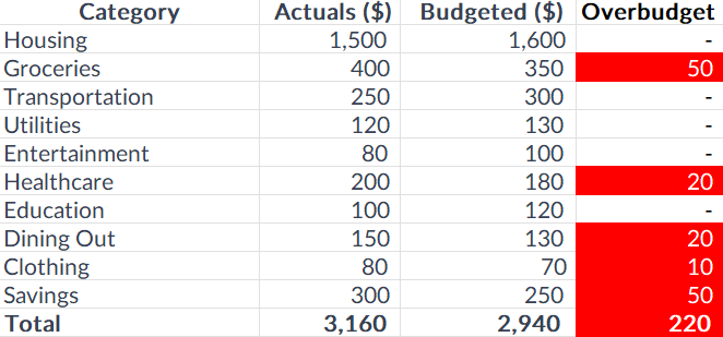
It’s a simple and effective way to alert your eyes to amounts that show a category is overbudget. But you don’t have to be limited to just changing colors.
Adding symbols to your conditional formatting
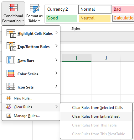
Instead of changing cell and text colors, I’ll simply add a red flag next to an amount when it is overbudget. First, I’ll clear off the conditional formatting rules I’ve already created. You can remove rules one by one or you can just delete all of them. To do that, go to the Conditional Formatting button and this time select the option to Clear Rules and to Clear Rules From Entire Sheet.
Now the conditional formatting is gone and I can start over. But before I do that, I need to find the symbol that I want to use in the custom formatting. If you go to the Insert tab, off to the right there is an option for Symbols.

By clicking on that, you’ll see many different symbols you can insert into your spreadsheet. If you scroll around you can find symbols that look like flags, which is what I’m going to use.
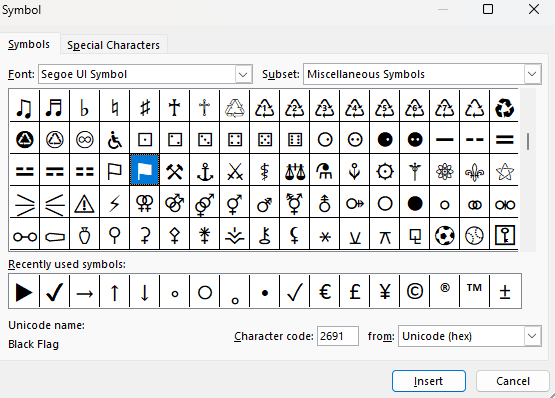
The one that I have highlighted above is for a Black Flag. I can click on Insert to put it into my spreadsheet.

To get this symbol into my custom format, I first need to copy it. To do that, double-click on the cell so that you are editing it, and then select the flag, and then press CTRL+C to copy. While it’s copied and in the clipboard, now is the time to setup the conditional formatting rules. The process is the same as before.
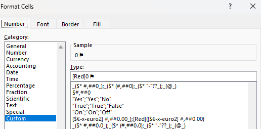
Except this time, when it comes to applying the custom formatting, go to the Number section, and select Custom. Then, enter a value of 0 and then paste the flag symbol. If you want to also highlight everything in red, you can add [Red] in front. Here’s what that custom number format could look like:
After applying the rule, now the table looks like this, with the custom formatting:
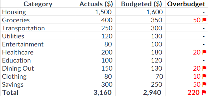
This is a bit of a cleaner format that you can use rather than having to highlight the entire cells. You can use this approach for other symbols in Excel. The key is just to find the symbol you want to use and then copy and paste it into your custom format.
If you liked this post on How to Add Flags to Conditional Formatting Rules, please give this site a like on Facebook and also be sure to check out some of the many templates that we have available for download. You can also follow me on Twitter and YouTube. Also, please consider buying me a coffee if you find my website helpful and would like to support it.

