

Creating a Pivot Table is one of the fastest ways to summarize large amounts of data in Excel. But if your data is spread across multiple sheets, it can seem a little overwhelming. The good news is: you don’t have to manually copy everything into one sheet. You can easily combine multiple sheets into a single Pivot Table.
In this Excel tutorial, I’ll walk you through how to make a Pivot Table from multiple sheets, step-by-step, with the help of Power Query. If you want to follow along, download the practice file here.
Loading the data into Power Query
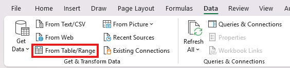
You will need to have your data setup in tables in order to combine all of it. However, you can do that all at once. Go through each tab and select your data, and under the Data tab, click on the option to get data From Table/Range:
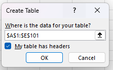
Excel will automatically detect your range. You can adjust if need be, otherwise, you just need to confirm whether it contains headers (which it should to avoid issues later on):
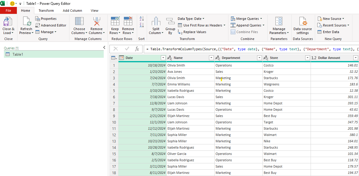
This now opens up Power Query, where your data is now visible:
On the Home tab, select the option for Close & Load and select Close & Load To and choose Only Create Connection.
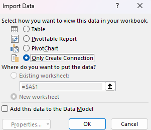
This ensures the data is added into Power Query but it does not create a new tab. Repeat these steps for the other tabs.
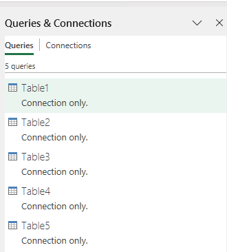
If you forget to select the option to only create a connection, then you can just delete the tab that is created afterwards; the result is the same — only a connection will be created. After loading five tables in this practice file and creating the connections, you should see the following queries under the Queries & Connections pane on the right-hand side (this should automatically display when you first add a table to Power Query).
With the data loaded, now let’s go into Power Query by right-clicking on any of these connections and selecting Edit.
In Power Query, on the left-hand side, you can edit the table names so that you know what they relate to:

By right-clicking on the table names, you can change them. I’ve renamed them so that it is clear which regions they relate to:
- Table1: Northwest
- Table2: Northeast
- Table3: Southwest
- Table4: Southeast
- Table5: Central
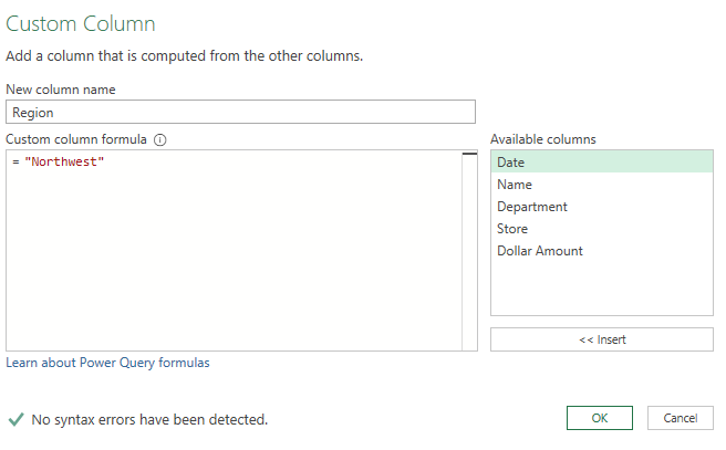
In each table, I’m also going to add a field called Region, where I will list the names of those tables. By going into the Add Column tab and selecting Custom Column, I can enter in the new column name as well as the value. This is the custom column I’m creating for the Northwest table:
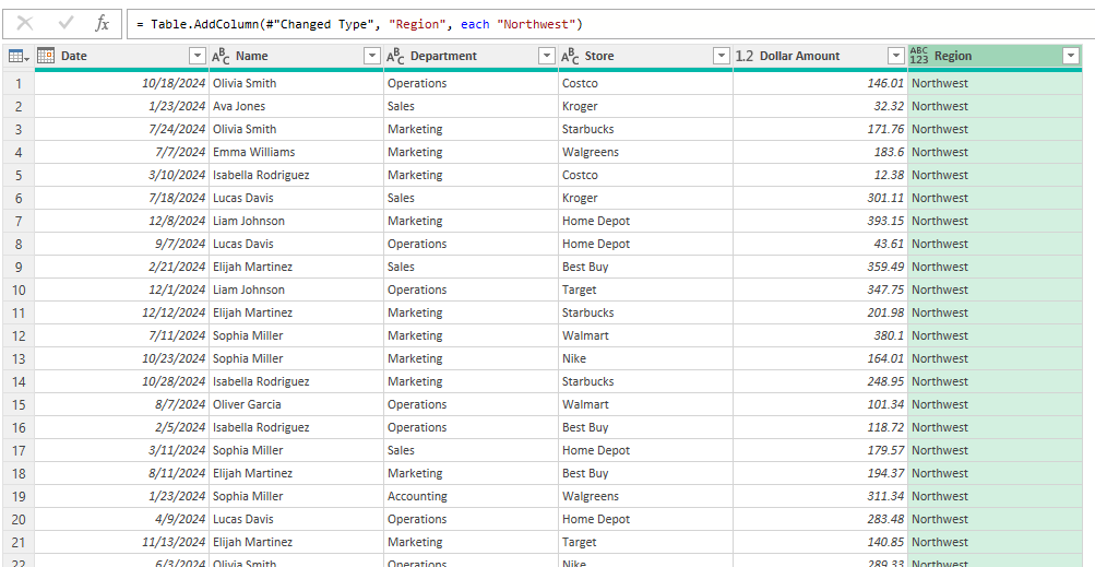
After creating the column, this is what the updated table looks like:
Repeat these steps for the other tables, entering their specific regions for the Region field. In order to ensure the data is consolidated correctly, you’ll want to ensure that the field names are the same.
Appending the queries together
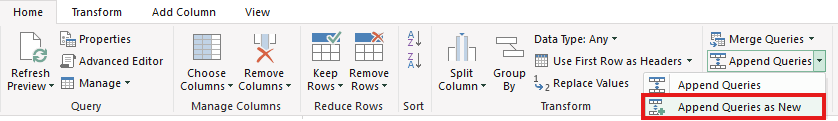
With all the data in Power Query, we can append the queries together, to create one large table. To do this, go to the Home tab and select the Append Queries as New option, which will create an entirely new query:
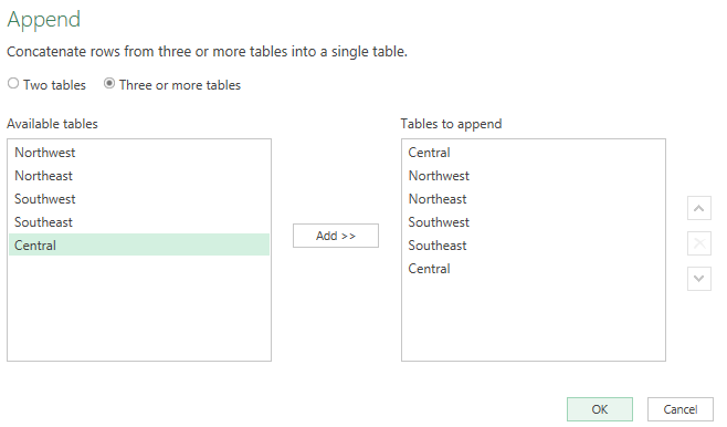
Select the option to append three or more tables and select all of them and then click OK:
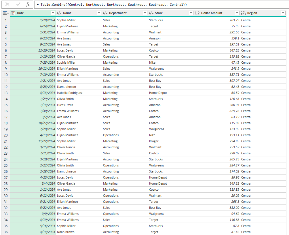
Now, all the tables are appended into one query:
Now, this appended table can be loaded into Excel. In this instance, you don’t want to create just a connection but instead download the entire table into Excel.
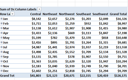
This table can now be used to create a Pivot Table as you normally would, through the Insert -> Pivot Table option. And now, when creating your pivot table, you’ll see the values from all regions combined. You can now slice the data based on region and month, and whatever other fields are in the data set.
If you enter more data and want to update your pivot table, what you first need to do is go to the Data tab and click on Refresh All. This will refresh your queries. You will also need to do another refresh to ensure that the pivot table updates after that. This can be done by just right-clicking on the pivot table and clicking refresh rather than doing Refresh All again, which will also update the queries and may be more time consuming.
If you liked this post on How to Make a Pivot Table From Multiple Sheets in Excel (Step-by-Step Guide), please give this site a like on Facebook and also be sure to check out some of the many templates that we have available for download. You can also follow me on Twitter and YouTube. Also, please consider buying me a coffee if you find my website helpful and would like to support it.