
Creating a pivot table is not difficult to do. If you just go to the Insert menu in Excel, there is an option to select a Pivot Table. As long as you have your data selected, Excel goes to work and creates the table. But making a good pivot table is an entirely different story. And that’s the real challenge — making your pivot table easy to read and understand, and not cumbersome to update. To help you with that process, here, I’ll list 10 of the most common mistakes you can make when creating a pivot table, and how you can avoid them!
1. Not cleaning your data beforehand
The old adage of “garbage in, garbage out” is true when it comes to data analysis, and pivot tables are no exception. If you have data that has incorrect values, then there’s no sense in creating a report on it. Take the time to check and review your formulas, make sure you don’t have any blank or missing values (or at least keep them to a minimum), and also check for spelling inconsistencies. That last one can be an easy one to miss. If you have a value with an extra space, that won’t be the same as a value without one.
If you spend the time of cleaning up and reviewing your data before you create a pivot table, you’ll save yourself some headaches and possible embarrassment later on; no one wants to provide their boss with a report that is incorrect.
2. Forgetting to use an Excel table
To convert your data into a table is easy — just use the CTRL+T shortcut. By doing so, you’ll ensure that your table will automatically expand and your formulas will copy down as you add new entries and rows. And as long as you pivot table references your table, then you won’t have to worry about re-adjusting the range later on. Otherwise, if you’re referencing a static range, the danger is that you forget to include new data as you add on to it. And in that situation, your report may once again be incorrect.
3. Not refreshing after data changes
Even if you’re using a table, you still need to ensure that your pivot table is refreshed. Unless you have a macro setup, this is a process you’ll need to do manually. By right-clicking on your pivot table and clicking Refresh, your data will update. You can also go to the Data tab and select Refresh from there.
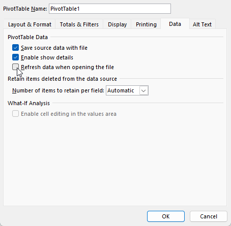
Alternatively, if you right-click and select Pivot Table Options, under the Data tab, you can choose to Refresh data when opening the file, which will do a refresh when first opening the file.
4. Using merged cells in source data
Merged cells can cause lots of issues in Excel, including with pivot tables as that can cause problems when grouping your data. If you have merged cells, that can also mean that values are missing from certain fields. Merged cells should generally be avoided in Excel, and even if you want to spread a title across multiple cells, as you might with a header, there’s an easy way to look as though you’re merging a value without actually merging the cells.
5. Dragging text fields into the values area
If your pivot table looks like this, where you have a count of values when you’re expecting to see a summation or an average, it’s likely that you’ve put a text value in the values section:
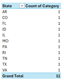
This happens because Excel doesn’t know what to do with these values since it can’t add them. In the above example, a text field (category) has been placed in values section and upon doing so, Excel simply does a count of them. To fix this, ensure that you are correctly organizing your pivot table and not putting any text fields into the values section.
6. Not renaming field labels
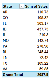
When creating a pivot table, you might be tempted to leave the default names when setting it up. However, that can lead to unnecessarily long titles such as Count of Category or Sum of Sales.
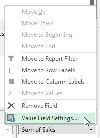
You can fix this by selecting the arrow next to the pivot table field and clicking on Value Field Settings:
You might be frustrated that you can’t change the name to the same label. If I were to change the field to simply say ‘Sales’ then I would get an error stating that it’s already in use since that is the source name. However, an easy workaround is to just add an extra space. By renaming it to ‘Sales ‘ it no longer triggers an error and in the pivot table, it will look as though I’ve used the same name as the source. It also saves space and can make your field names more meaningful; there’s no reason you have to use the defaults.
7. Using Inconsistent Date Formats
If your dates are not entered as dates, and some are reading as text, or perhaps are entered as day/month/year rather than month/day/year, this can be another problem, because it can mean your data isn’t being grouped correctly.
This can be a harder issue to catch and that’s where doing a spot check of your pivot table after it has been created is helpful. You can clean your data beforehand, but errors like this are more difficult to spot. This is why it’s always a good idea to review your pivot table, and make sure it makes sense. If you have sales in a future month, for example, that can be an easy way to spot that you have a possible problem with your dates.
8. Repeating the same layout changes over and over again
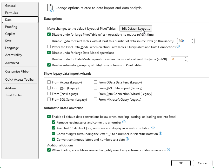
When you first setup a pivot table, the default layout may not be what you want. But instead of making the same changes over and over again, why not simply save them as your new default? Once you’ve made the changes that you want, such as repeating labels and/or displaying the pivot table in a tabular format, you can save your pivot table layout as a default. This can be done by going to File-> Options -> Data and selecting Edit Default Layout for your pivot table.
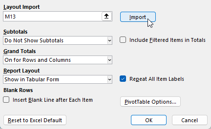
You can import the layout by just selecting the pivot table you’ve modified and clicking on the Import button.
9. Making changes to individual cells rather than fields
One frustrating and easy-to-make mistake is to format pivot tables the way you might regular tables and other data in Excel. You might be tempted to select an entire column and change the formatting to how you want it. The problem? Once your pivot table refreshes, the data reverts back to its previous form. This is happening because you aren’t adjusting the underlying field settings.
To adjust the actual field, select it from your pivot table layout and go into Value Field Settings. Once there, go into the Number Format option and make any formatting changes there.
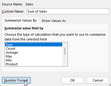
Now once you make the changes, they will remain intact, even after you update your pivot table.
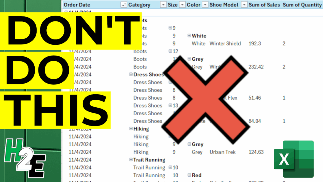
10. Overcomplicating the Layout
As easy mistake to make with a pivot table is by cluttering it up with too many fields. In the below example, I have too many fields listed in the Rows section, and they’re in an order which isn’t logical, going from category->size->color->shoe model.
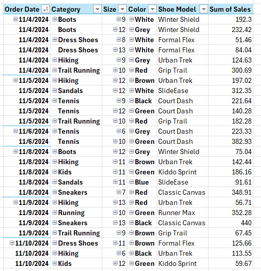
This doesn’t make the pivot table easy to read and understand. I have almost recreated the original table by setting it up this way. A good mix involves putting some fields in the rows section and some in the columns. And a good rule of thumb to follow is to use the fields which contain the most number of items in the rows section, rather than columns. This is because it’s a lot easier to scroll up and down with a mouse wheel versus horizontally and having to drag the scroll bar.
If you liked this post on 10 Pivot Table Mistakes to Avoid, please give this site a like on Facebook and also be sure to check out some of the many templates that we have available for download. You can also follow me on X and YouTube. Also, please consider buying me a coffee if you find my website helpful and would like to support it.