

A VLOOKUP function in Excel can be an effective and easy way to pull in a value from a list. But what if you needed to base your lookup on multiple values? You could use helper columns to try and achieve that, but there’s another way you can do so, and it involves the LOOKUP function, which is similar to VLOOKUP, but it gives you a bit more flexibility.
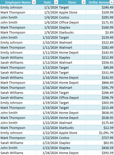
For this example, I’m going to use the following data set, which has a list of expenses by employee.
The LOOKUP function takes the following arguments:
- lookup_value
- lookup_vector
- results_vector
I’m going to create a couple of lookup fields, specifically for the employee name, date, and store. My formula is going to check the table against each one of these fields, with the goal being that any time the criteria is a match, a value of 1 is returned. Here’s what my criteria will look like when I’m looking for a combination of date, employee name, and store:
((Table1[Employee Name]=employeefield)(Table1[Date]=datefield)(Table1[Store]=storefield))
Where employeefield, datefield, and storefield are the values in my spreadsheet that I’m looking up that pertain to these specific columns. If there is a match, a value of 1 is returned each time. And so if all the criteria are met, then it becomes 1 x 1 x 1 = 1. If any one of the criteria is not met, however, then 0 is returned since anything multiplied by a 0 is a 0.
But I don’t want to return 0s and instead I want the values to be errors so that they don’t affect the result. To do this, I’m going to take 1 and divide it by all the above criteria. That way, if there is a 0 value, it returns a #DIV/0! error. This is what this portion of my formula looks like at this point:
1/((Table1[Employee Name]=employeefield)(Table1[Date]=datefield)(Table1[Store]=storefield))
The third part of the function requires the results vector to pull the values from. In this example, it’s the Amount field:
((Table1[Employee Name]=employeefield)(Table1[Date]=datefield)(Table1[Store]=storefield)),Table1[Dollar Amount])
Finally, for the first part of the formula, is the actual lookup value. I’m going to be searching for a value of 2, since that will ensure it pulls in the last match (in case there are multiple), as all the values will either be errors or 1 values. This is what the complete formula looks like:
=LOOKUP(2,((Table1[Employee Name]=employeefield)(Table1[Date]=datefield)(Table1[Store]=storefield)),Table1[Dollar Amount])
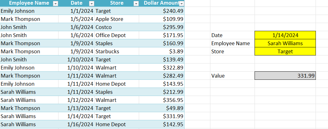
And here is how it all looks within my spreadsheet, with the input fields in yellow and the result in grey (which is where the above formula resides):
If you liked this post on How to Do a Lookup in Excel With Multiple Criteria, please give this site a like on Facebook and also be sure to check out some of the many templates that we have available for download. You can also follow me on Twitter and YouTube. Also, please consider buying me a coffee if you find my website helpful and would like to support it.