
Conditional formatting rules can help highlight values and identify when certain criteria is met. You can also create advanced rules that include formulas. And I’ll walk you through how to to do so in a way where it’s easy to test your logic and ensure you setup your rules correctly.
Start with creating a formula in your spreadsheet
You might be tempted to jump right into the conditional formatting settings and create your rules. But you’re probably better off not doing that, because if you need to make an adjustment later on, it can be challenging to try to tweak the formula there.
Instead, start with creating a formula within your spreadsheet. The goal is to setup a formula so that it results in either a TRUE or FALSE result. If it’s TRUE, then your conditional formatting will get applied. Otherwise, it won’t.
In the below example, I’m using the NFL prediction template I created earlier. If you want to follow along, download that template and delete the conditional formatting rules that are already there.
I’m going to create a rule to track if teams I’m interested in are playing. If they are, I want to highlight those games.

In this template, I have a section for a watchlist, starting in row 14. I’m going to select a few teams I want to track.

This watchlist is in the range A14:A21. I need to create a conditional formatting rule that meets two conditions:
- If the home team is found in the watchlist, or
- If the away team is found in the watchlist.
While this doesn’t sound complex, creating the conditional formatting rule for this can be a bit of a challenge. A good way to set this up is to create a formula in an adjacent column to see if it is calculating correctly.
Let’s start by using the MATCH function. This function will search through the watchlist to see if it finds the lookup value.
=MATCH($E4,$A$14:$A$21,0)>0
Column E is where the home team is listed. I’ve frozen column E since the search criteria shouldn’t change, regardless of which cell I’m in. This is important to ensure the entire row is highlighted.
Currently, how this formula works is if a value is found on the watchlist, it will result in a value of 1 or more, and that will return a value of TRUE. However, if the team isn’t found, then the formula results in an #N/A error. To fix this, I’m going to put the entire formula within the IFERROR function:
=IFERROR(MATCH($E4,$A$14:$A$21,0)>0,0)
Next, I need to also setup the formula to check if the away team is found in the watchlist. This is the exact same formula, except instead of referencing column E I’m referencing column I, which is where the away team is listed.
=IFERROR(MATCH($I4,$A$14:$A$21,0)>0,0)
Now, I’ll combine the two formulas within the OR function:
=OR(IFERROR(MATCH($E4,$A$14:$A$21,0)>0,0),IFERROR(MATCH($I4,$A$14:$A$21,0)>0,0))
Now, I’m going to copy this formula down to confirm it is calculating correctly:
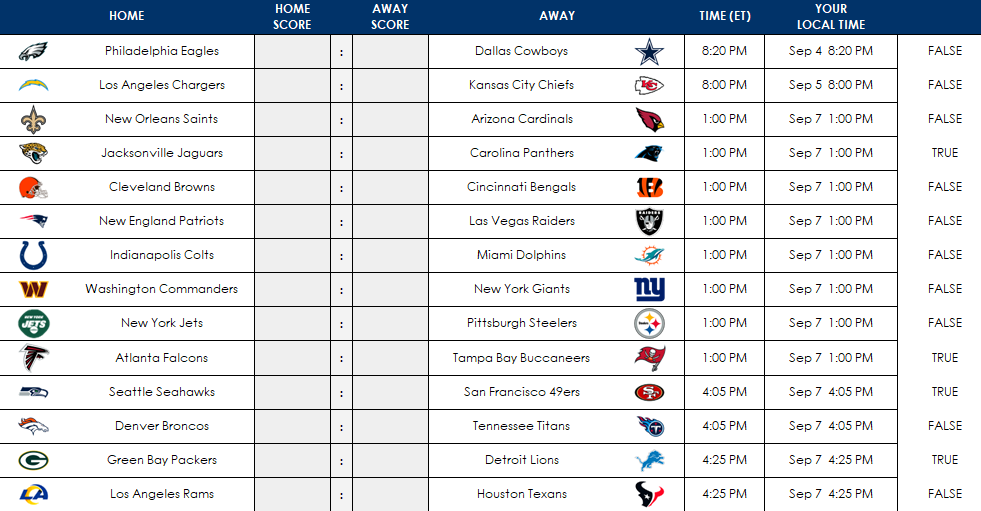
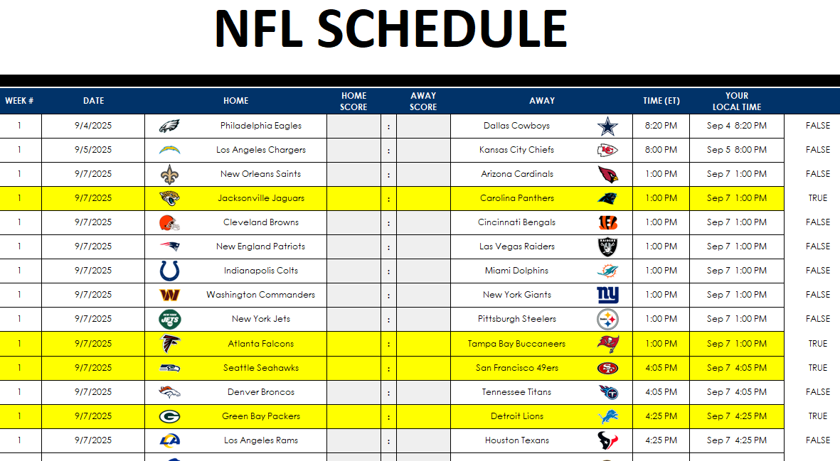
On the right-hand side, you can see the values being returned as either TRUE or FALSE. And the TRUE values are showing for the teams in my watchlist (Carolina, Tampa Bay, Seattle, and Green Bay). This confirms that the conditional formatting rules are setup correctly.
Adjust the starting range for your conditional formatting formula
When I initially setup the conditional formatting rules I referenced row 4, since that was where the first game was. But when I setup my conditional formatting rule, I need to change it to row 1, since I’m going to select columns B:L, and thus, I need to start from row 1 to ensure my conditional formatting is not being offset by any number of rows.
Thus, the formula I’m going to copy into the conditional formatting is as follows:
=OR(IFERROR(MATCH($E1,$A$14:$A$21,0)>0,0),IFERROR(MATCH($I1,$A$14:$A$21,0)>0,0))
Create the conditional formatting rule
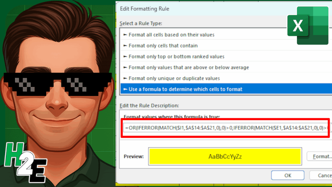
With columns B:L selected, I’m going to go into the Conditional Formatting menu and select New Rule. And I’m going to select the option to use a formula, which is where I will paste the above formula into:
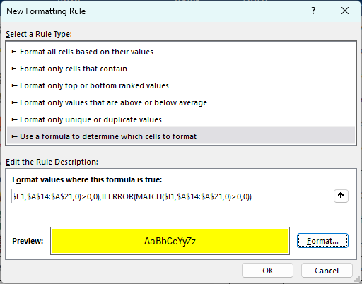
I have also set the formatting so that the fill color is yellow and the font color is black. Now, I’ll click on OK. Initially, it looks as though my conditional formatting rules are incorrectly applied:
Double-check your conditional formatting rule and change it if necessary
I’m going to go back into the conditional formatting settings, where I see Excel has modified my starting row:
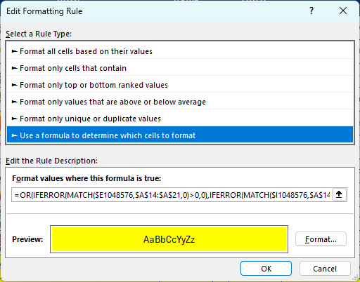
Since I selected the entire columns, Excel has selected the very last row, 1048576, which is clearly not what I wanted. This can happen when you select an entire column and so it’s always important to go back in and double check the formatting once it has been setup. I’m going to have to manually go into here and adjust the formula so the first cells in the MATCH functions are $E1 and $I1 again.
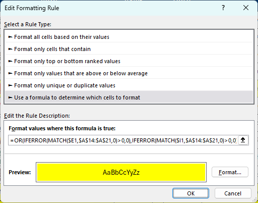
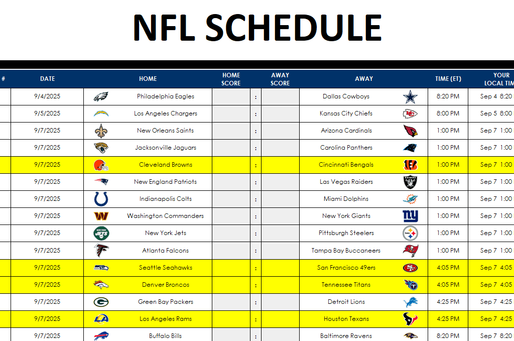
This is a one-time fix that’s necessary. And after doing so, now I can see that my conditional formatting is correctly applied, and the values that show TRUE in the far right column are indeed highlighted.
With the conditional formatting correctly applied, I can now clear the formulas I setup earlier in the column that is checking if the condition is met (where the TRUE and FALSE values are showing).
To use formulas in conditional formatting, it’s a good idea to first test your logic within your spreadsheet. That way, it’s easier to confirm it’s evaluating correctly and easier to make adjustments as necessary.
If you liked this post on How to Setup Advanced Conditional Formatting Rules in Excel Using Formulas, please give this site a like on Facebook and also be sure to check out some of the many templates that we have available for download. You can also follow me on Twitter and YouTube. Also, please consider buying me a coffee if you find my website helpful and would like to support it.