In a previous post I have gone over how to use LEFT and MID functions for parsing data, but in this post, I’ll go through a specific example from start to finish.
I am going to pull my data from the citymayors website, url as follows:
http://www.citymayors.com/features/capitals.html
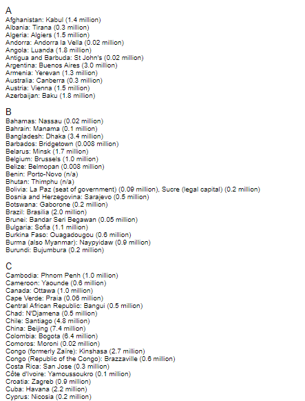
The data on this page looks like this:
At first glance, this isn’t the most useful data that you can paste into an Excel spreadsheet but I’ll show you how it can be made more usable. First off I will copy the entire data set into a spreadsheet.
It copies in much the same as how it looked on the webpage. The problem is it is not in a format that you can do any analysis on. The structure it currently follows is Country: City (population). The more consistent the data is, the easier it is to pull the information out. In this sample, there are some inconsistencies but for the most part, it follows a logical pattern.
I am going to make the following columns: Country, City, and Population.
I’ll start with the Country column. For this field, I can use the LEFT function. However, the country names range in length so I can’t simply take the first x amount of characters. Instead, I have to look at where the colon shows up and stop one character before that.
I am going to start will cell B2 to analyze cell A2. In order to find the colon, I can simply use the FIND function. The formula for this will look as follows:
=FIND(“:”,A2,1)
I insert this formula into the LEFT function so that I get the following
=LEFT(A2,FIND(“:”,A2,1)-1)
What this formula does is look at cell A2, and pull characters until one before the colon (since I don’t want to actually include the colon). I will make one additional adjustment to avoid errors and that is if the cell in A2 is fewer than two characters it will return a blank (rather than an error since it would not find a colon). The formula to check for a length greater than two characters is this:
LEN(A2)>2
Inserted into my earlier formula:
=IF(LEN(A2)>2,LEFT(A2,FIND(“:”,A2,1)-1),””)
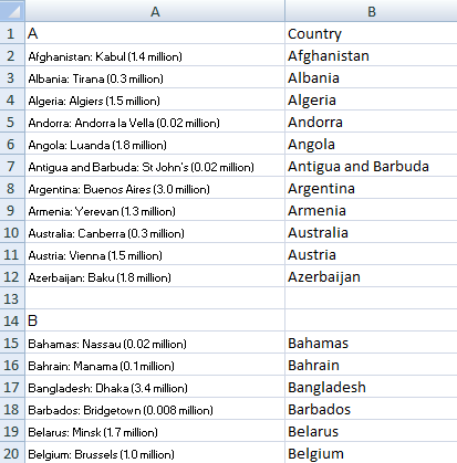
This qualifies the cell first by saying only if it is more than two characters long will my formula try to pull data out, otherwise, it will leave it as blank (“”). I will copy this formula all the way down my country field. This is what my spreadsheet looks like now:
Next up is the City field. This one is going to be a bit more difficult because I can’t start from the left and have to use the MID function where I will need to search for both the colon (my starting point) as well as the bracket that starts the population field (my ending point). In the MID function, I need to specify the start and endpoint, whereas with the LEFT function it started from the first character in the cell.
The first formula I need to make is to get my starting point. But I’ve already done that in the country field, I can just copy the FIND formula from earlier:
FIND(“:”,A2,1)
In this case, I will want to add +2 to the end of it so that it skips over the blank space after the colon and starts at the first character of the city name. My formula currently looks like this:
=MID(A2,FIND(“:”,A2,1)+2
Next, I need to find the endpoint, and similarly, I can use the FIND function to find the opening of the parentheses. The formula for this is similar to my earlier one:
=FIND(“(“,A2,1)
I will want to subtract two characters from this so that I do not include the open parenthesis character or the empty space before it. If I insert this formula into the MID function I now have the following:
=MID(A2,FIND(“:”,A2,1)+2,FIND(“(“,A2,1)-2
The problem with this is finding the ( character does not tell me how long the city field is. To get the actual length of the field, I need to subtract the starting point of the field, which is again using the earlier formula to find the colon. My adjusted formula looks like this:
=MID(A2,FIND(“:”,A2,1)+2,FIND(“(“,A2,1)-2-FIND(“:”,A2,1))
I will add the same qualifier to check for a length of two or more characters. My updated formula:
IF(LEN(A2)>2,MID(A2,FIND(“:”,A2,1)+2,FIND(“(“,A2,1)-2-FIND(“:”,A2,1)),””)
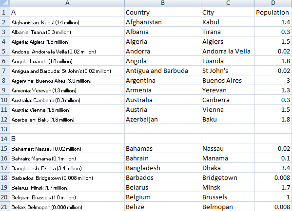
If I copy this formula down my spreadsheet now looks like this:
Next is the population field. Again I will use the MID function and I can use the endpoint of the city field as the starting point for my population field. I am only going to extract the numbers because numbers with text are not useful for analysis. If I wanted to I could pull the million text into another column and then could adjust the numbers accordingly. However, in this instance, it looks like all the figures are in millions so it is not necessary.
My formula starts as follows with the MID function and the previous formula to find the ( character:
=MID(A2,FIND(“(“,A2,1)+1
I added the +1 again so that it starts from the number rather than the ( itself. Next, I need to find the length so I need an endpoint for which I can use the FIND function again. This time I can just look for the empty space that comes after the number. So far I have the following:
=MID(A2,FIND(“(“,A2,1)+1,FIND(” “,A2,1)
The ” ” indicates a blank space. The problem here is I cannot start from the first character because it will find the first space. If the country has a space it will return a value from there, and if not there it will pull the space that comes right after the colon. What I need to do is change the value of 1 to where the ( is found. The updated formula:
=MID(A2,FIND(“(“,A2,1)+1,FIND(” “,A2,FIND(“(“,A2,1))
This will now make sure it retrieves the first space after the ( character, which is what I want. I could have made it simpler and just looked for the word ‘million’ but that would not work for instances where the word did not show up (and I also wanted to show a more complicated example). Next, I need to subtract the starting point so that the length is correctly calculated:
=MID(A2,FIND(“(“,A2,1)+1,FIND(” “,A2,FIND(“(“,A2,1))-FIND(“(“,A2,1)-1)
I deducted one at the end because I did not want to include the space after the number. However, there is still one problem. Even though I extracted a number it is still text. I can convert it to a number simply by multiplying the result by one:
=MID(A2,FIND(“(“,A2,1)+1,FIND(” “,A2,FIND(“(“,A2,1))-FIND(“(“,A2,1)-1)*1
Now the number aligns to the right of the cell, indicating it is a number rather than text (which aligns to the left). I will add my qualifier for the length of the cell:
=IF(LEN(A2)>2,MID(A2,FIND(“(“,A2,1)+1,FIND(” “,A2,FIND(“(“,A2,1))-FIND(“(“,A2,1)-1)*1,””)
Unfortunately the data set is not perfect and in some cases there are text in parentheses so I would want to correct any of those cells – which should be easy to find since they result in errors. Alternatively, I could in the meantime use an IFERROR function to make any errors result in a 0 value:
=IFERROR(=IF(LEN(A2)>2,MID(A2,FIND(“(“,A2,1)+1,FIND(” “,A2,FIND(“(“,A2,1))-FIND(“(“,A2,1)-1)*1,””),0)
Copying the formula to all the cells my spreadsheet now looks like this:
Using the IFERROR allows you to make the data usable for data analysis. And at the same time because you wouldn’t expect a population to be 0, you can still easily find error cells.
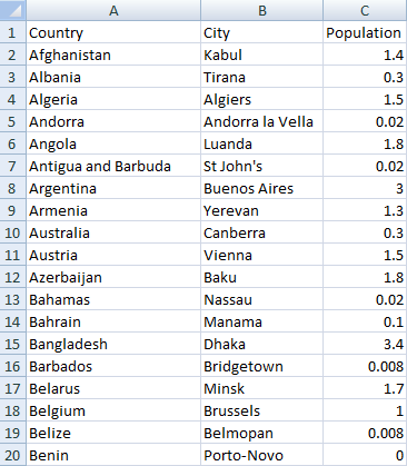
Once you are done parsing your data, I suggest copying and pasting it as values. This ensures you are not dependent on the original data. Once you have done that you can also eliminate any blank values in the Country, City, or Population fields. This will allow you to have an unbroken data set that you can easily filter or use in a pivot table. My completed data set after these changes looks like this:
The key thing to remember is that the original data needs some consistency in it before you can use a formula to be applied to it. If there is no consistency or has a lot variations to it, the more complicated your formula would need to be to pull what you need from it. In those situations, I prefer to use Visual Basic just because of the complexity that may be involved. This data set was fairly consistent and still involved some long, complex formulas to extract data from it.


[…] an error. To pull the values that are needed to arrive at a proper date value, we’ll need to parse the data. Parsing can be a bit complicated but when you’re dealing with text, it’s the […]