How to Do a Vlookup and Extract Multiple Columns

VLOOKUP is a powerful function for extracting data from another sheet. And while most users will use it simply for pulling just one field, it can do a lot more than just that. Below, I’ll show you how you can extract multiple columns from just a single vlookup formula, potentially saving you from having to repeat the same formula over and over when you need more than one field.

Let’s start with the basics

First, I’ll setup a regular vlookup formula and then show you how, with a simple adjustment, you can pull a lot more data into your spreadsheet.

For this example, I’m going to use data from NationMaster, showing the number of vehicles in use by country. In addition to raw numbers, the data set also shows the year-over-year growth and the five-year compounded annual growth rate (CAGR). Here’s what the data looks like in my Excel sheet:

In a normal vlookup formula, you might have something like this setup if you wanted to extract all of the fields:

Cell H4 is where I’ve entered the country name. The vlookup works just fine if you want to pull data from the vehicles column. And if you want to grab the other fields you can just repeat the formula for the YOY% and 5-Year CAGR fields and just change the column number. However, there’s a much easier way to extract all those fields using just one formula.

Modifying the VLOOKUP formula

All I need to do to make this formula accommodate multiple columns is to change the column number. Rather than this:

=VLOOKUP($H$4,$A:$D,2,0)

I’ll enter in this:

=VLOOKUP($H$4,$A:$D,{2,3,4},0)

Using the curly braces, you can specify the different column numbers that you want to extract. Since this is an array formula, on older versions of Excel you may need to enter ALT+SHIFT+ENTER for the calculation to work properly.

Here’s the difference in formulas:

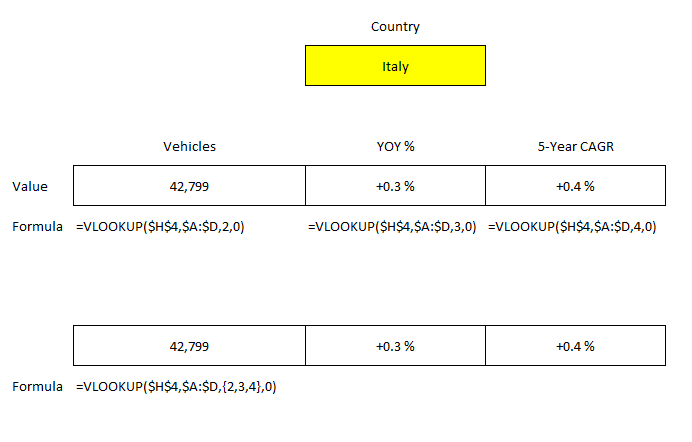
The columns you want to extract also don’t need to be sequential. You can extract columns 2 and 4 rather than all three. All you need to do is separate the column numbers that you want with a comma.

Retrieving the fields vertically instead of horizontally

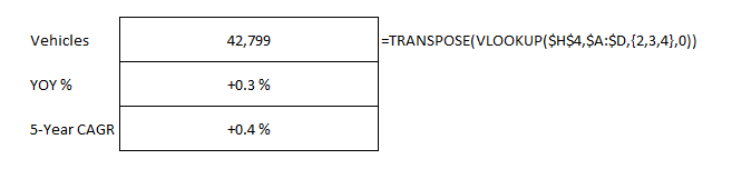
Depending on how you’ve got your sheet set up, you may prefer for the data to come back in rows rather than columns. This too, is an easy fix.

All that you need to do is wrap your existing formula within the TRANSPOSE function. Here’s what the updated formula looks like:

=TRANSPOSE(VLOOKUP($H$4,$A:$D,{2,3,4},0))

This again is an array formula so you may need to use CTRL+SHIFT+ENTER on older versions of Excel. But doing it will allow you to retrieve the values vertically:

There’s a lot of flexibility with how you can use vlookup to extract data that can allow you to not only simplify your spreadsheet but also result in having to create fewer formulas.

If you liked this post on how to extract multiple columns from vlookup, please give this site a like on Facebook and also be sure to check out some of the many templates that we have available for download. You can also follow us on Twitter and YouTube.