If you’ve ever downloaded data and received dates in the wrong format, it can be a challenge to fix. If your regional settings are month/day/year but in a spreadsheet they are in day/month/year format, then odds are they will be reading in a text format rather than date. The one exception is when you’re dealing with month and day values that are 12 or less, and thus, they could be both month or day values. In those cases, the values are still reading as dates, but they are still incorrect. Here’s how you can fix all of these issues by using a formula.
Converting text date formats using TEXTSPLIT and INDEX
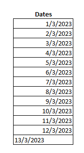
Suppose you have the following values, which are for March 2023:

These dates are not in the month/day/year format. However, only the value that has a 13 at the start is aligned to the left — indicating that it’s a text value. The others are recognized as dates, even though they are in the wrong format. This is what can make this calculation tricky, to accommodate both situations — but it’s not impossible.
First, let’s deal with the values that are in text. For these ones, their values just need to be parsed out. In the past, you could do this with a complicated series of LEN, MID, LEFT, and RIGHT functions. However, thanks to the relatively new TEXSPLIT function, it’s easier to do that.
Here’s how you would parse out the data if it’s in a text format, such as in the last instance (March 13), which is in cell A14:
=TEXTSPLIT(A14,”/”)
This formula will break out the data into an array:

This isn’t the final solution, as this would still require another formula to pull these values into a date. And to accomplish that, this is where the INDEX function comes into play. Since there are three values here, using INDEX, you can select which value goes in which argument for the DATE function.
For instance, the following formula would extract the first value before the /, which is the number 13:
=INDEX(TEXTSPLIT(A14,”/”),1,1)
For the second number, 3, the column argument needs to change to a 2, to get the second column in the array:
=INDEX(TEXTSPLIT(A14,”/”),1,2)
And for the last one, the column would be set to 3:
=INDEX(TEXTSPLIT(A14,”/”),1,3)
Together, these values can be put within a DATE function. The arguments in the DATE format are in the following order: year, month, day. That means that last value in the array (position 3) needs to be first, followed by the second position (the month), and the last position (for the day). Here’s how that formula looks:
=DATE(INDEX(TEXTSPLIT(A14,”/”),1,3),INDEX(TEXTSPLIT(A14,”/”),1,2),INDEX(TEXTSPLIT(A14,”/”),1,1))
It’s the same formula repeated but referencing different column positions. And now, the formula gives me the date in the correct month/day/year format:

However, this formula won’t work on the other values; they will result in errors since those are date values and only display slashes but don’t actually contain them the way a text value does. However, the solution for these formulas is even easier.
How to rearrange date values
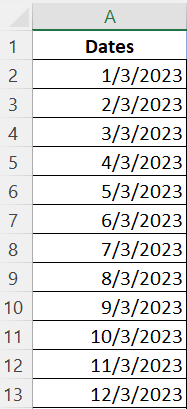
Since the below cells read as date values, we can reference their respective month, day, and year values, and simply put them back into the DATE function.

The first value is the day value, followed by the month, and then the year. However, my regional settings are set to month/day/year format. That means if these cells are reading as date values, which they are, then that means the first value is going to be the month. By using the MONTH function, I can get that first value. But the key is, when I’m creating a new formula and using the DATE function, I will need to put that value in the argument that relates to the day. This can be a bit tricky and remember, if your regional settings are different from mine, you will need to alter your formula to ensure the right value is going into the right argument.
Similarly, for the second value (which corresponds to the day in my regional settings), I will use the DAY function to get that value. But I will actually put it in the month argument.
Lastly, the YEAR function will extract the year and go into the same year argument position, since month/day/year and day/month/year have the same position for the year. Here’s how this formula looks in its entirety, grabbing all the different values:
=DATE(YEAR(A2),DAY(A2),MONTH(A2))
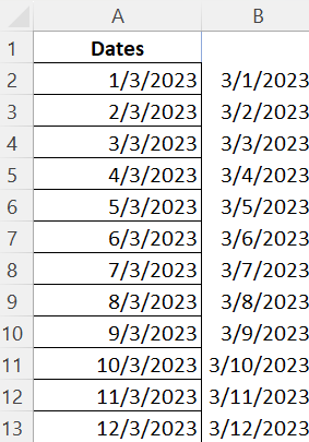
By copying the formulas, the date formats now look correct:

Combining the formulas
There’s just one left piece left in all of this, and that’s combining the two formulas so they can accommodate both situations: when the data is in text format, and when it’s reading as a date. This can be done by using the ISTEXT function, to check if a value is reading as text or not. If it’s a text value, then it will use the TEXTSPLIT function. Otherwise, it will simply reposition the date values. Here’s the formula that will factor in both situations:
=IF(ISTEXT(A2),DATE(INDEX(TEXTSPLIT(A2,”/”),1,3),INDEX(TEXTSPLIT(A2,”/”),1,2),INDEX(TEXTSPLIT(A2,”/”),1,1)),DATE(YEAR(A2),DAY(A2),MONTH(A2)))
Now, this one formula can be used on all of the cells, whether they are in date or text format.
If you liked this post on How to Convert Date Formats in Excel, please give this site a like on Facebook and also be sure to check out some of the many templates that we have available for download. You can also follow me on Twitter and YouTube. Also, please consider buying me a coffee if you find my website helpful and would like to support it.

