Do you have multiple lists in Excel or Google Sheets that you want to combine together? With new functions such as VSTACK and HSTACK, you can do just that. In this post, I’ll show you how you can also filter out duplicates and apply sorting so that your data is organized after consolidating all of your lists.
Combining multiple stock lists into a large one
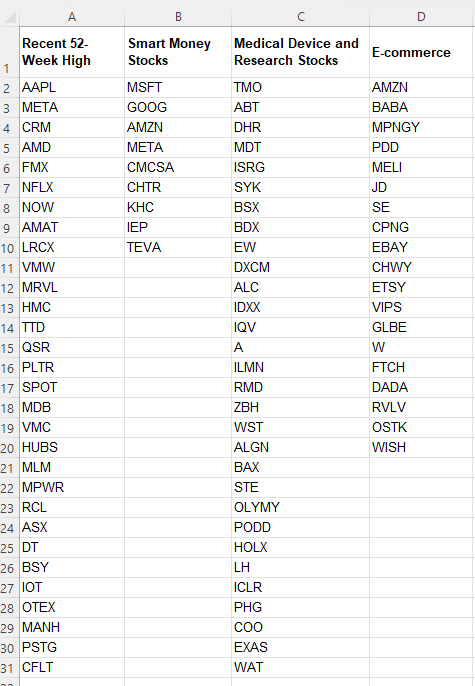
In this example, I’ll use various stock lists that I want to combine into one large list. On Yahoo Finance, you can find an assortment of different lists to help filter stocks. Below, I’ve pulled the lists of stocks that recently hit new 52-week highs, smart money stocks, medical device and research stocks, and e-commerce stocks:

The advantage of keeping the lists separate is that you can more easily update them. And by using VSTACK, you can combine these lists into a larger one so there’s no worry about having to consolidate them later on.
Based on the lists above, this is the formula that I use to combine them all together, using VSTACK:
=VSTACK(A2:A31,B2:B10,C2:C31,D2:D20)
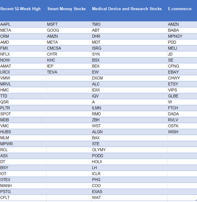
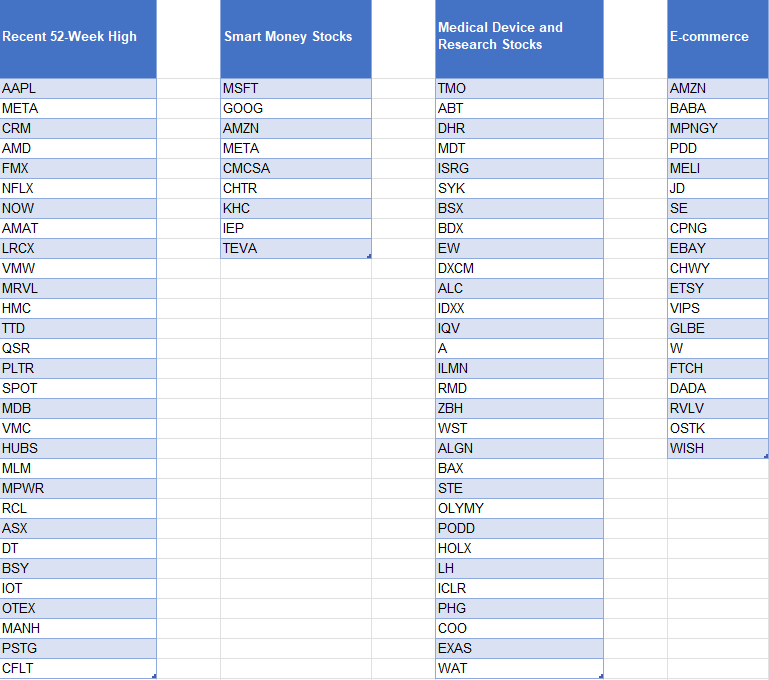
Since I don’t want to include the headers, I start from row 2. You’ll notice that I’ve hardcoded the ranges here. One way to make this more dynamic would be to use a COUNTIF or COUNTA function for the individual lists, and then use the INDIRECT function to limit the scope of the list. Another option involves converting the lists into tables. That way, you only have to list the table column and you don’t have to worry about the ranges. The one caveat here is that if you have lists that have different lengths, you’ll want to make each list its own table. Otherwise, Excel will automatically fill in the gaps with blank values:

While the data looks correct, if I were to use the VSTACK formula for these different table columns, I would get a consolidated list that involves many zero values. To keep it cleaner, it’s easier to just separate them into their own tables, and then reference them afterwards.

To reference these columns, my formula becomes much simpler:
=VSTACK(Table1[Recent 52-Week High],Table2[Smart Money Stocks],Table3[Medical Device and Research Stocks],Table4[E-commerce])
The advantage of doing it this way is that now I don’t have to worry about hardcoding the ranges, and thus, it’s easier to update.
Whichever method you prefer, the end result should look like a consolidated list:

Removing duplicates and sorting the list
In some of these lists, there is some overlap. AMZN and META are two stocks that show up twice. This means that my consolidated list will include those values multiple times. To get around this, I can embed the formula within the UNIQUE function:
=UNIQUE(VSTACK(A2:A31,B2:B10,C2:C31,D2:D20))
If you also want to sort your list, then you can add the SORT function as well:
=SORT(UNIQUE(VSTACK(A2:A31,B2:B10,C2:C31,D2:D20)))
Use HSTACK for horizontal arrays
If you have the same lists but instead have them going horizontally, then you can use the HSTACK function. It works the same way as the VSTACK but as the H suggests, it will require horizontal arrays. Here are the same list of stocks as in the first example, this time transposed so that they go horizontally:

In this case, the formula for HSTACK would be as follows:
=HSTACK(B1:AE1,B2:J2,B3:AE3,B4:T4)
You can apply the same steps as for the VSTACK to eliminate duplicates and to sort the results.
These formulas work the same in Google Sheets as in Excel
Whether you’re working in Google Sheets or Excel, these formulas will be the same. The VSTACK, HSTACK, SORT, and UNIQUE functions are all available on the latest version of Excel and on Google Sheets. There is no need to change any of the formulas besides just adjusting for any difference in ranges. The formulas themselves work in the same ways, making it easy to transfer data between Google Sheets and Excel and to replicate these formulas wherever makes sense for you.
If you liked this post on How to Use VSTACK and HSTACK in Excel and Google Sheets to Consolidate Lists, please give this site a like on Facebook and also be sure to check out some of the many templates that we have available for download. You can also follow me on Twitter and YouTube. Also, please consider buying me a coffee if you find my website helpful and would like to support it.

