If you work on large teams and/or interact with people all over the world, you know it can be challenging trying to work with time zones. While they aren’t difficult to understand, it’s easy to make a mistake when trying to arrange a meeting, as one time might seem like it works well only to discover later on that it’s during an inconvenient time for another person. Office software like Microsoft Outlook can help with this, but you can also setup a template in Excel or Google Sheets to convert time into different time zones. In this post, I’ll show you how you can setup an easy-to-use template that can calculate these differences for you.
Creating a template to convert time into other time zones
To quickly convert time from one time zone to another, the key piece of information you need is the Greenwich Mean Time (GMT) offset. Once you know this, then it’s a matter of just making of using simple arithmetic to convert from one time zone to another.
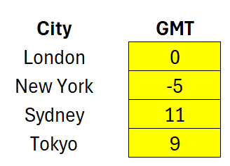
Let’s suppose your home city is London. There is no adjustment needed as its offset is 0. For New York, the adjustment is -5, and for Sydney it is +11, and Tokyo is +9. This is during non-daylight savings times. Positives can be left without an indicator but for negative adjustments, we need to put in a negative value in front to ensure the conversions are calculated correctly.

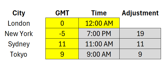
Let’s assume London is my base time, and I sent it to 12:00:00 AM. To determine the total adjustment in hours, I need to compare to the two GMT adjustments. To convert from London to Sydney is simple as I just need to add 11 hours, and in the case of Tokyo, 9 hours. New York is a bit trickier since that is behind London — hence the negative value. To make it work with the TIMEVALUE function, I need the value to be positive. Whether I deduct 5 hours or simply add 19 hours (24-5), I end up with the same time. This means, when there is a negative difference, I can just add 24 hours. That results in my GMT hours adjustment formula looking like this.
=IF(B3-$B$2<0,B3-$B$2+24,B3-$B$2)
Where B3 is my New York GMT offset and B2 is my London GMT offset.
Next, to convert the time, I’ll use the TIMEVALUE function. This can be done with taking that time zone hours adjustment from the previous step, and putting it within the TIMEVALUE function, and adding it to my base time.
=$C$2+TIMEVALUE(D3&":00")
Where D3 is the adjustment from my previous step and C2 is my base, or home time. These calculations work the same whether you’re setting this up in Excel or Google Sheets.
You can re-use this template to do different conversions based on various parts of the world. With the correct GMT adjustments for each city, the calculations can easily be updateable.
In the screenshot below, I’ve highlighted any inputs in yellow and formulas in grey to help show how a user can modify the template to do time zone conversions.

I don’t have to use London as my base city and instead I can switch it around to New York. I can also change it so that my starting time is 7:00 PM New York time. The results will be the same, and it’s just the adjustment value that changes.

If you like this post on Converting Time Zones in Excel and Google Sheets, please give this site a like on Facebook and also be sure to check out some of the many templates that we have available for download. You can also follow me on Twitter and YouTube. Also, please consider buying me a coffee if you find my website helpful and would like to support it.

