Excel’s what-if-analysis options aren’t the greatest, but one option which is very useful and can save time is Goal Seek. What Goal Seek effectively does is it can do trial and error for you in seconds, and be much more precise than doing it manually.
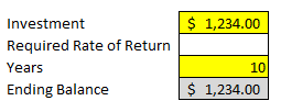
In many examples you could use algebra to get to your answer but if it’s a one-time calculation perhaps it’s not worth the trouble of going that route. For example, suppose I had an investment of $1,234 and wanted to know what average return would be needed for it to grow to $10,000 after 10 years. This can certainly be done with algebra, but Goal Seek can also do it. Below, I have entered my inputs in yellow.
My ending balance is equal to the following formula : =C4*(1+C5)^C6
C4 = Investment
C5 = Required Rate of Return
C6 = Years
Next, I will select Goal Seek from the Data tab under What-If Analysis
The next screen prompts me to enter which cell I want to set to which value, and which cell I want changed to accomplish this (the variable). In my example I use C7 for the set cell box (this is my desired ending balance), the value is 10,000, and by changing cell I enter my required rate of return (which is C5).
After clicking OK it fills in the required rate of return as 0.23273147. It also sets the value in C5 to this amount as well. If I hit OK on the next screen the value in C5 will keep this value, if I cancel, it will revert to what was there before – nothing.
This was a simple example but there are also more complex ones it can be used for. Another example could be an amortization table. The table below has a principal amount owing of 10,000, an interest rate of 5%, a payment of 550 per month. This is what it looks like:
So it will take roughly 19 payments to for this amount to be paid off under the terms described. But let’s say I wanted to know precisely what interest rate would have to be applied to make the ending balance at payment number 20 equal 0. I don’t want an extra payment for the balance to be included at the end, just so that it perfectly matches 0 after payment 20.
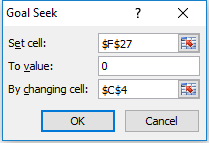
To do this, I go back to Goal Seek. For the first box (set cell) which is what I want my result to be – I select the ending balance at payment 20 – currently it is (579.34). This is cell F27 on my spreadsheet. The second box is what result I want, which in this case is 0. Lastly, my variable, or the cell I want changed to make this work – that is my interest rate, which is in cell C4 – currently it is at 5%. These are what my inputs look like:
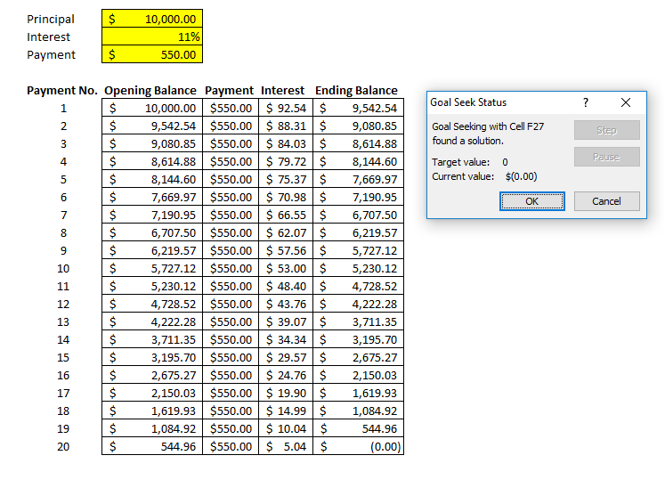
Once I hit OK, I get the following:
You’ll notice now my target value matches my current value and the Goal Seek was successful. It has changed my interest rate to 11% – not exactly 11%, 11.1048262490731%. A very precise percentage that has allowed my table to reach 0.
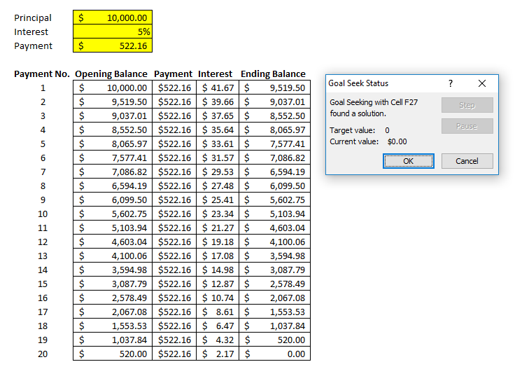
Goal Seek can be used in a variety of different circumstances as you can see. As long as you have a formula like in the above two cases that the change cell (e.g. variable) directly effects, then it should work. I could have selected the payment as my change cell rather than the interest rate and my result would be as follows:
It would indicate a rounded payment of 522.16 (exact amount of 522.162995552194) would be needed to pay off after 20 payments with the interest rate staying at 5%.
The one limitation of Goal Seek is that you can only use one variable. But beyond that it does it very well and can help save you a lot of time.


Add a Comment
You must be logged in to post a comment