How to Combine Two Columns in Excel

If you’ve inherited or downloaded a data set, you know that sometimes you’ll need to combine data together to make it in the format that you want. A good example is a list of addresses where you may have the street information in one column and the zip or postal codes in another column. To get all the information in one cell would require combining the information. Below, I’ll show you multiples ways of how you can combine two or more columns in Excel.

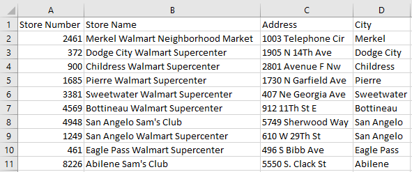
My data set for this example includes some sample address information on Sam’s Club and Walmart locations in the U.S. :

Using the ampersand to combine columns together

The easiest way is to join the cells through a simple formula. The easiest way to do so is by using the ampersand (&). In column D below, I’ve joined the cells and in column E is the formula that I’ve used:

This gets the job done but you’ll notice a small issue: there isn’t a space between the information. that makes the data a bit messy and it’s probably not what you want. But it’s an easy fix. It can be addressed by adding another ampersand between the cells and add open quotes ” ” to add a space. This is how my spreadsheet looks after I’ve made those changes:

This can be expanded to more than just two columns. If I wanted to add the store name field (column A) into the mix, then it’s just simple as adding another ampersand for the field and another one for another extra space. Here’s how the data looks like all three columns joined together:

This can start to become a bit cumbersome as you add more fields into one cell. An alternative way that you may find easier if you’re working with several columns is using the CONCATENATE function.

Using the CONCATENATE function

The CONCATENATE function works very similar to how the ampersand. However, it’s a bit cleaner in that you don’t have several ampersands in your formula. If you wanted to group cells A2, B2, and C2, your formula would look like this:

=CONCATENATE(A2,B2,C2)

If you want a space to be included between each of those fields, then it looks like this:

=CONCATENATE(A2,” “,B2,” “,C2)

Here’s how that would look if I applied it to my existing data set:

You can use commas to separate the data if you prefer and in that case, you would just use “,” instead of an empty quote. You can also add extra spaces in between quotes to space out your data even further.

But whether you choose to use the ampersand or the CONCATENATE function just comes down to preference. Either approach can get the job done.

If you liked this post on how to combine cells in excel, please give this site a like on Facebook and also be sure to check out some of the many templates that we have available for download. You can also follow us on Twitter and YouTube.