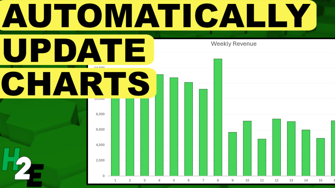
When you add data to an Excel spreadsheet, with regular charts, you often need to trigger a refresh to make sure that your chart reflects the latest data. But, by using Power Query, you can automate that process without the need for macros. In this post, I’ll walk you through the process of getting your data into Power Query, and how to set it up so that your charts will update automatically.
Step 1: Importing Data into Excel with Power Query
The first step involves pulling data into Power Query. This can be from various sources like databases, web pages, or local files. In this example, I’m just going to use data that’s on another sheet, but it can also be from another workbook. Here is an excerpt of some sales data since the start of the year:
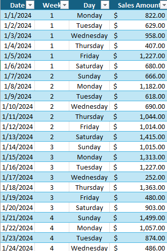
To get this into Power Query, I just need to click on any of the cells in the table and then under the Data tab, under the Get & Transform Data section, select the From Table/Range option. Now my data is in Power Query.
But before loading the data back into Excel, I’m also going to group the totals by week. To do this, I’ll click on the Group By option in the Home tab in Power Query. I’ll create a column name called Weekly Total and sum the Sales Amount:
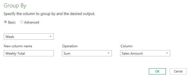
Now I have sales broken down by week which I can import back into Excel.
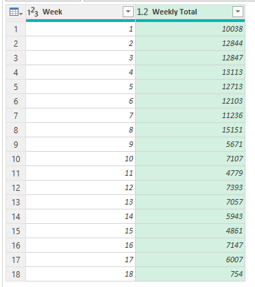
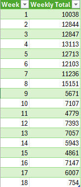
At this stage, I’ll click on Close & Load. Now I have another table of the data in Excel, this time, linked to Power Query and broken out by week:
Step 2: Creating a Chart from Imported Data
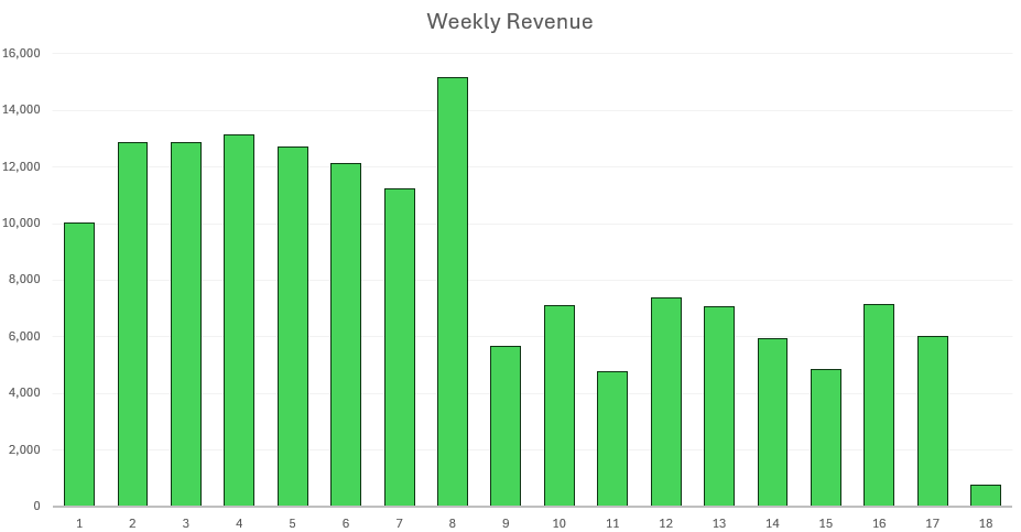
Next, let’s go ahead and create a chart to show these daily sales totals. For this example, I’ll use a simple column chart showing the weekly sales. To do this, click on your data set anywhere and on the Insert tab, select the option for a Column Chart. After applying some formatting, this is what my chart looks like:
Step 3: Setting Up Automatic Refresh
With my chart and table now setup, I can go ahead and set the automatic refresh. When a query is created in Power Query, you will see it under the Queries & Connections pane. To show this pane, go under the Data tab and click on Queries & Connections. Then, right-click on the query and select Properties. You’ll now see the following options:
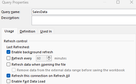
As you can see, there is an option to specify how often you want to refresh the data. You can have it refresh when you click on the Refresh All button but you can also set it to refresh when the file first opens. And you can even specify it to refresh every few minutes. I can even set it to refresh every minute:
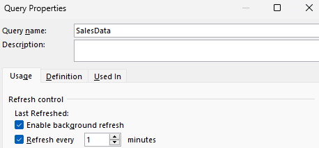
Depending on how often your data may change, you may want to adjust this accordingly. But one thing to keep in mind is that whatever changes you made in Power Query, refreshing the query will trigger all those steps, which can make it time consuming if there are many steps for the query to go through.
But by setting up a rule to refresh every x number of minutes, you can have control over how often your data updates. And since it’s linked to a chart, your chart will also automatically update.
If you like this post on How to Automatically Update Your Excel Chart With New Data Using Power Query please give this site a like on Facebook and also be sure to check out some of the many templates that we have available for download. You can also follow me on Twitter and YouTube. Also, please consider buying me a coffee if you find my website helpful and would like to support it.

