

Is your pivot table not updating even though you’re refreshing the data? If that’s the case, that usually means there’s a problem with the data that your pivot table is referencing. Here’s how you can troubleshoot and fix the issue. Note: If your pivot table is linked to power query, you’ll want to first review that your query is updating correctly before moving forward.
Check your pivot table’s data source
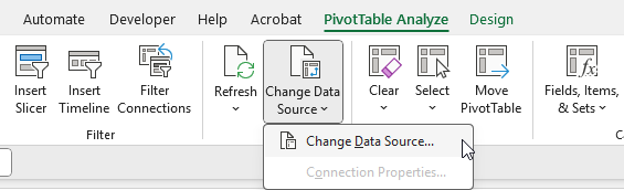
The first thing you’ll want to do when you’re looking into problems with your pivot table’s data, is to start by going straight to the source. Click anywhere on your pivot table, as doing so will display the PivotTable Analyze tab on the ribbon. If you click in here, you’ll see an option to Change Data Source. Even though you may not necessarily want to change the data source, this is where you can see where your pivot table is pulling data from.
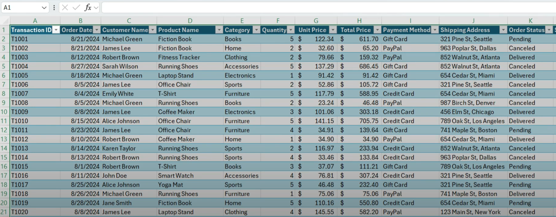
When you click on the button to change the source, you’ll see the table or range that your pivot table is referencing. In this example, it’s referencing the range A1:L150 in the Sales_Transactions tab:

If your data goes beyond the range, that’s where your problem exists. In my example above, the pivot table range only goes to row 150, but my data goes all the way to row 201.
Since the pivot table has a hardcoded range, anytime I add data beyond row 150, this pivot table will not include it, even if I do a refresh. The band-aid solution is to simply update the range to go to row 201. I could set a larger number for the row to give myself more of a buffer, but the danger is always that the pivot table may not be optimally sized, and the risk is that not all of the data will be included even when a refresh is done.
When creating pivot tables, the ideal solution is to put your data in a table
To avoid the issue of a pivot table refresh not updating your data, the best option is to put your data into a table. Once in a table, your range will automatically update, and you no longer need to worry about how many columns or rows to include; the table will expand as you add more data.
To create a table, click anywhere on your data set, and go to the Insert tab, where you’ll see a button for Table. By clicking this button, Excel will create a table and auto-detect your range. By default, it’ll also applying some formatting so that you’ll recognize it’s in a table format. But you can also change the color scheme of your table if you prefer.
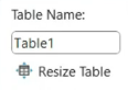
Once you create a table, Excel also assigns a name to it. If it’s the only table in your sheet, you might see a name such as Table1 in the Table Design tab, under the Table Name field:
This reference now becomes a named range that you can use when creating or updating a pivot table. Rather than a fix ranged of cells, the pivot table can simply reference the table. And after making this change, any data that is added to the table will be included when the pivot table refreshes.
Creating a named range without a table
You don’t have to create a table to setup a dynamic named range for your data set, but it’s the easiest option. Another way is to create a named range that uses the OFFSET Function, which can automatically adjust based the number of rows and columns.
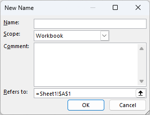
This is a more complicated setup, but how it works involves setting up a named range. Start by going to the Formulas tab and clicking on Name Manager. Then, click on the button for New, which will allow you to create a new name, and specify what range it refers to.
For the OFFSET function, you’ll need to also use the COUNTA function to count the number of non-blank rows and columns. Start by setting cell A1 as your starting position, and here is what the full formula will look like:
=OFFSET(A1,0,0,COUNTA(A:A),COUNTA(1:1))
This formula starts in cell A1 (which is where the pivot table begins in my example), doesn’t offset any rows or columns (the first two zero values indicate this), and then it counts the number of non-blank rows and columns, ensuring that it automatically expands. If you’re using this approach, you’ll want to make sure you have no other tables or data on the sheet, to ensure the COUNTA function is not picking up additional columns or rows, and expanding your range too far. And to keep it simple, I suggest putting your pivot table in cell A1.
Once you’ve created this named range, you can now use it as the data source for your pivot table, and it will do the same job as the table in that it will automatically expand as you add data.
If you liked this post on How to Fix a Pivot Table That Is Not Refreshing, please give this site a like on Facebook and also be sure to check out some of the many templates that we have available for download. You can also follow me on Twitter and YouTube. Also, please consider buying me a coffee if you find my website helpful and would like to support it.