

PIVOTBY is a relatively new function that Excel introduced in 2021. It is a dynamic, formula-based alternative to pivot tables. It’s part of Excel’s push toward more dynamic, flexible data analysis, especially for users who prefer formulas over the drag-and-drop interface of traditional PivotTables. In this article, I’ll walk you through what PIVOTBY does, how to use it, and provide some examples to help you master it.
What Does the PIVOTBY Function Do?
PIVOTBY summarizes data based on one or more grouping columns and returns an array with calculated values—similar to a pivot table, but directly inside a formula.
It allows you to group data by categories (like region, product, or date) and then apply an aggregation function (like SUM, AVERAGE, COUNT, etc.) on another column. Here are the main arguments for the function:
PIVOTBY(row_fields,col_fields,values,function,[field_headers],[row_total_depth],[row_sort_order],[col_total_depth],[col_sort_order],[filter_array],[relative_to])
Only the first four arguments are required:
- row_fields: this the range which will be used to group rows.
- col_fields: this is the range which will group the columns.
- values: this is a range for the data which is to be aggregated.
- function: this determines how the data should be aggregate (e.g. SUM, AVERAGE, COUNT)
How the PIVOTBY Function Works
Here’s a sample data set that I am going to use to illustrate how the PIVOTBY function works:
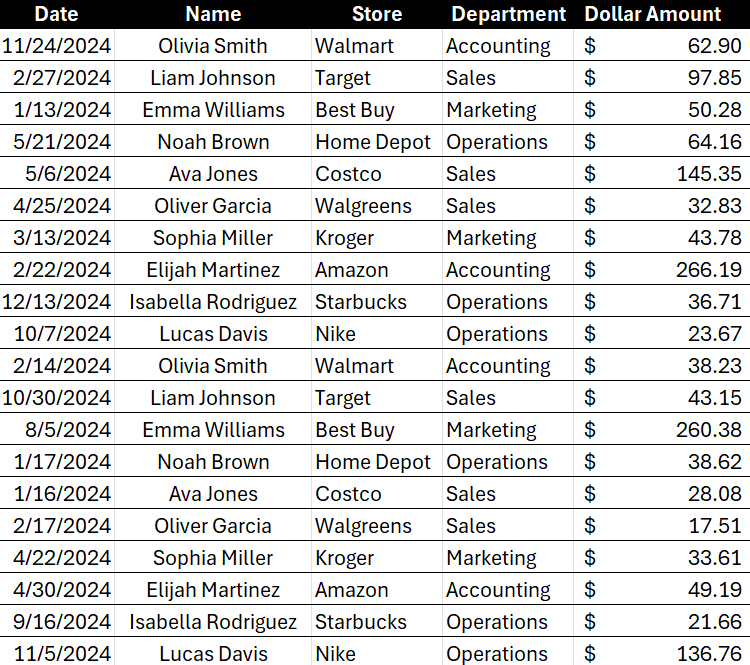
In the above table, dates are in column A, the name is in column B, followed by store in column C, department in column D, and amount in column E. Assuming my data is in a table called tblData, I can use the following syntax to create a pivot table showing sales by name and store:
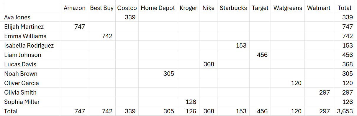
=PIVOTBY(tblData[Name],tblData[Store],tblData[Dollar Amount],SUM)
This produces the following values:
If you want to turn off totals for the rows, then you can set the row_total_depth argument to 0, as is the case below:
=PIVOTBY(tblData[Name],tblData[Store],tblData[Dollar Amount],SUM,,0)
And if you want both column and row totals off:
=PIVOTBY(tblData[Name],tblData[Store],tblData[Dollar Amount],SUM,,0,,0)
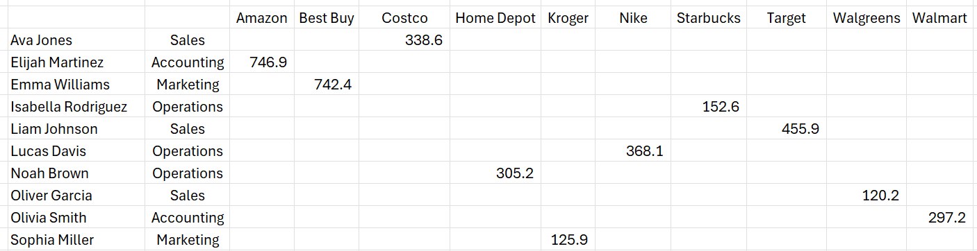
You can also pull in multiple columns or rows with the help of the CHOOSE function. Suppose you wanted to pull in both the name and the department a person is from. Here’s how you can accomplish that, while also removing totals:
=PIVOTBY(CHOOSE({1,2},tblData[Name],tblData[Department]),tblData[Store],tblData[Dollar Amount],SUM,,0,,0)
This produces the following report:
The benefit of this setup is that since this is a spill function, it will automatically update and populate the data and no refresh is necessary. There are, however, downsides to consider:
- If there is not enough space for the pivot table, you will encounter a #SPILL! error.
- Unlike a conventional pivot table, you can’t drill down to see the details
- This won’t work on versions of Excel prior to 2021.
If you just want an easy way to summarize your data without the need for drilling down, then the PIVOTBY function can work well and be a suitable replacement for a normal pivot table. For more of a comparison between the function your typical pivot table, check out this video:
If you liked this post on How to Use the PivotBy Function in Excel, please give this site a like on Facebook and also be sure to check out some of the many templates that we have available for download. You can also follow me on Twitter and YouTube. Also, please consider buying me a coffee if you find my website helpful and would like to support it.