How to Filter in Excel

If you’ve got a large data set, you know how important it is to be able to filter that data quickly and easily. Knowing how to filter efficiently in Excel can make it easy to not just pull up the data you need, but to also run calculations. Below, I’ll show you multiple ways that you can filter data.

For this example, I’m going to use a list of all the MLB World Series champions and runners-up.

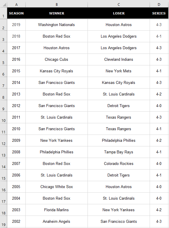
Using the auto filter

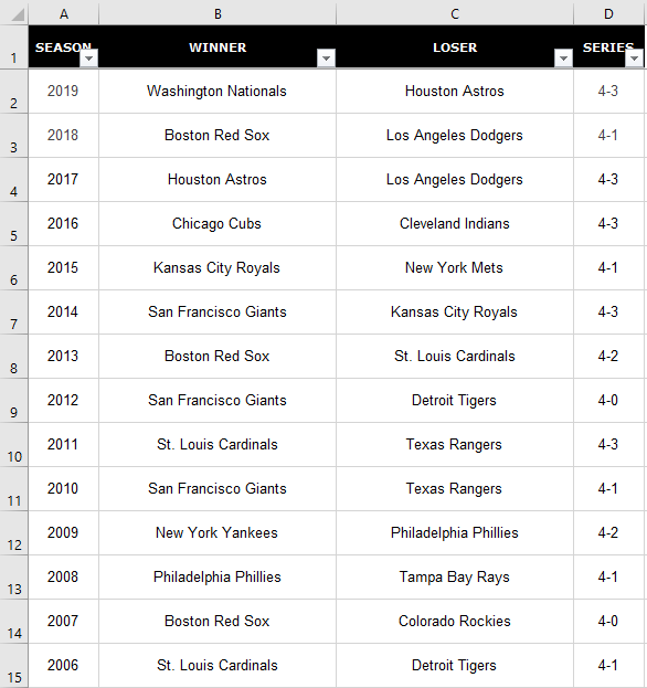
A quick way to filter the data is by using Excel’s auto filter. To enable it, click anywhere on the data set and click on Filter button from the Data section:

Clicking the button will create drop-down buttons that you can now use to filter the data with:

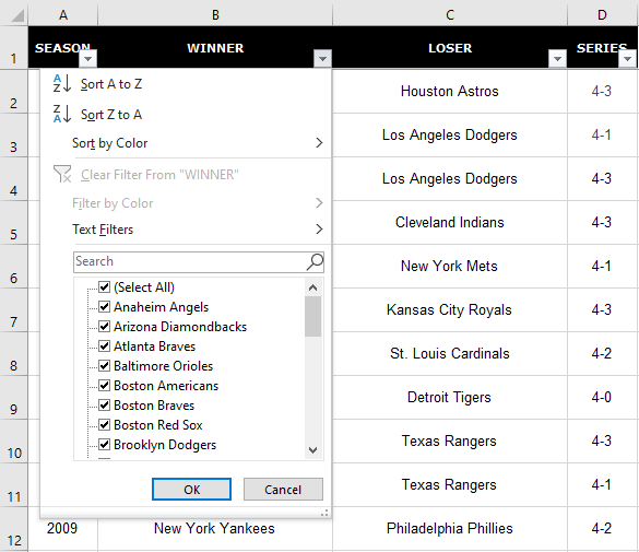
Suppose I wanted to see all the times that the New York Yankees have won. To do that, I would click on the drop-down button in the Winner column, where I’d now see all these options:

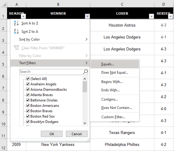
Filtering in Excel can be as easy or complicated as you want it to be. You’ll notice there’s even an option to Filter by Color that’s been greyed out since I don’t have any colors in my data set. If I click on the Text Filter option, I’ll have more options to choose from. I can look for partial matches and I can select an exact match as well:

In the following screen, I’ll enter in New York Yankees as my search term:

I can also have multiple criteria. For instance, I could say I want to see any victories by the New York Mets as well. In that case I could just enter another criteria and enter their name. However, there’as an even easier way to do that.

Although in the criteria, equals is selected, I can change that by clicking on the drop-down, and there I’ll have more choices:

I can select contains and just change the search criteria to New York. So even though I selected equals as my initial match criteria, I don’t have to worry about sticking to it. When I click OK, I now see my list of titles won by any team that had ‘New York’ in their name:

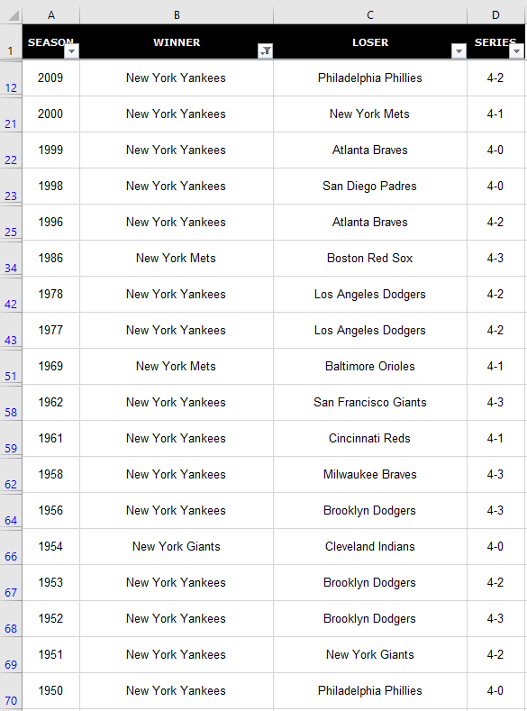
Not only do we have the Mets and Yankees on this list, but there’s also the New York Giants.

You’ll notice that the row numbers on the left are now in blue. This is how you can tell that your data is filtered. And so if you’re looking at your data set one day wondering why you’re missing information, have a look at the row numbers, as they may tell you the data’s filtered. If you want to unfilter the data, go back to the Filter button and click it again. Then your data set will be unfiltered and the drop-downs will be gone.

What you can also do is select the individual drop-down and clear the filter. You can tell which column has a filter in place by looking at the drop-down. In the Winner tab, the button shows a filter icon:

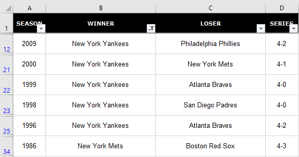
Clicking on that drop-down I’ll have the option to eliminate the filter:

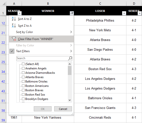
Clicking the Clear Filter From “WINNER” button will now reset the filter and keep the drop-down buttons in place.

Filter using selections

Using the text filter isn’t optimal because on newer version of Excel you see the list of items that you can choose from:

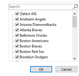
If I uncheck Select All and then scroll down to the New York teams and select them, I’ll arrive at the same result as if I did the text filter earlier:

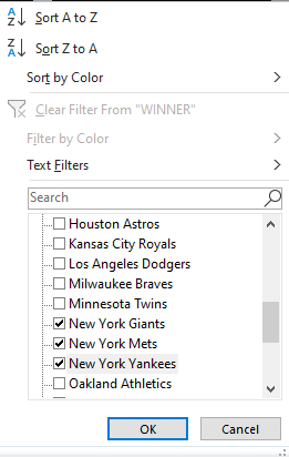
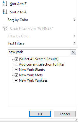
However, even this isn’t optimal. If I’m looking for a partial match, then I can just type in ‘New York’ in the search field and it’ll get the same selections:

There’s another less common way that you can filter data. If you’re just looking for one match, you can right-click on the value that you want to filter. Then, right-click on it and click Filter by Cell’s Value:

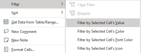
With this method, the drop-downs in the headers don’t have to be enabled. Once you run this filter, they will be there, however.

Filtering multiple combinations

It’s easy to filter when the names are similar. But if I wanted to filter the data for anytime a team from New York, Chicago, or Los Angeles has won, then it gets a bit trickier. One method would be to go back to the text filters and run multiple filters. But that’s an antiquated way of doing it. However, if you’re running an older version of Excel, that may be your only option.

If you can search through the filter, then there’s an easier way for you to do this. First, let’s go back to searching for ‘New York’ in the filter. We’ll again have all the New York teams in the list.

Next, let’s go back to the drop-down and search again. This time for ‘Los Angeles’ but before clicking OK, we’ll want to click off the box that says Add current selection to filter:

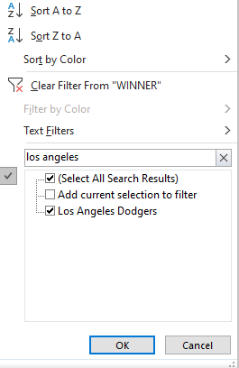
By default, this option isn’t checked. If I were to just click OK, the filter would be a list of Los Angeles teams only. But by checking off that box first and then clicking OK, I now have a list that contains both Los Angeles and New York:

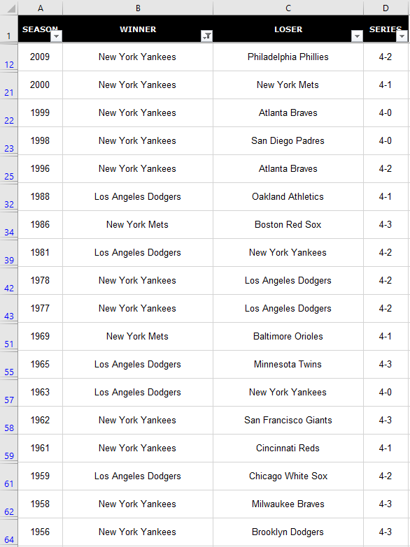
After repeating the process for Chicago I’ve now got all three cities in my list without having to go through the text filter:

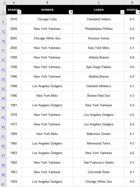
Use subtotals to make your filters even more useful

If I wanted to run a quick tally to see how many of the teams I’ve filtered have won a championship, I could use a COUNTIF function and enter their names. But if you want something more flexible where you can quickly run the filters as I’ve done above and see how many teams are in that list, you can use the SUBTOTAL function. The function takes in an argument for what type of calculation you want to do.

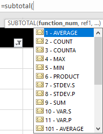
Now, since this data isn’t numeric, I’m going to use a COUNTA function, which is function number 3. For the range, I can use any column since it doesn’t matter which one I’m counting. But I will use range A2:A1000 because I don’t want to include the header in my total. Here’s how my formula looks like:

I could also use the MAX function to see the last time one of the teams I’ve selected has won. I’ll put that directly below the other formula:

Now, if I were to re-filter this data, this time, only for New York, my subtotals will automatically update:

The benefit of using the SUBTOTAL function is your data updates along with your filters. If you want the data to be static and not change, that’s when a regular COUNTIF function would be more appropriate.

If you liked this post on how to filter in Excel, please give this site a like on Facebook and also be sure to check out some of the many templates that we have available for download. You can also follow us on Twitter and YouTube.