How to Hide Zero Values on an Excel Chart

If you have values that you are plotting on a chart and some of them are zeroes, you will likely notice your chart sliding all the way down to the bottom. It can be problematic when you are entering in year-to-date data which will inevitably lead to blank or zero values. That’s why in this post, I’ll show you how to hide zero values from showing up on a chart in Excel.

Let’s start with the following example:

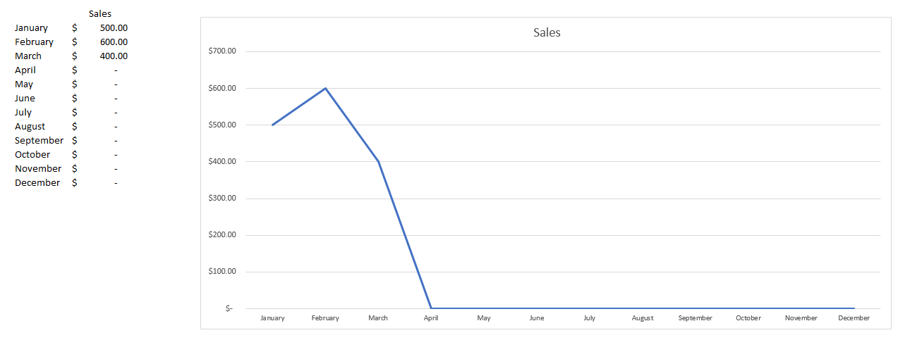
In this case, we have values for just a few months. From April through to December, the values aren’t necessarily zero — we just don’t have data yet. But the problem is that on the chart, the line graph shows them as being zeroes. If we were to get rid of those zero values, it would fix the issue:

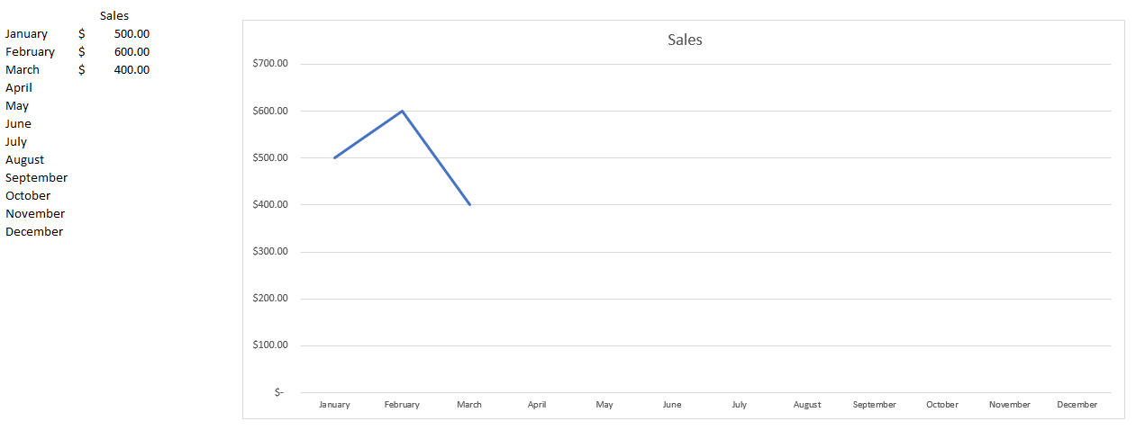
But the problem is that this may not be a convenient solution. If you want to create formulas to calculate the totals for each month, going back and deleting the ones with no values and remembering to put the formulas back in for future months isn’t going to be a very convenient option. There is a way that the calculations can be adjusted so that you can still get the zero values not to show.

Let’s suppose you have a SUMIF calculation for each month which looks as follows:

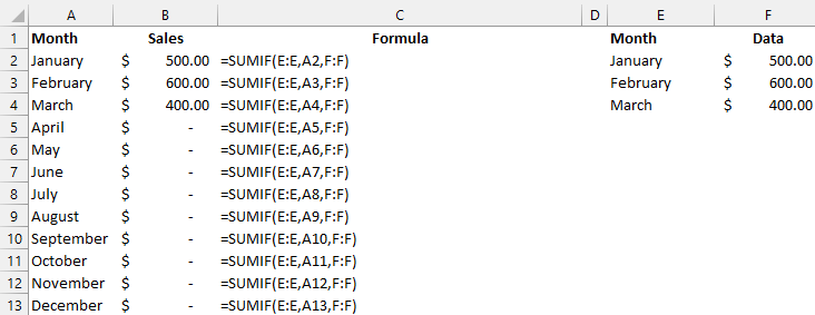
One way to fix this issue is to add an IF statement to avoid the zero values. But returning a blank value won’t fix the issue. Instead, what we’ll want to do is return an #N/A value. To do that, you just need to use the following formula:

=NA()

That just needs to be incorporated into the formula to say that if the sum is equal to 0, an NA value is returned:

=IF(SUMIF(E:E,A3,F:F)=0,NA(),SUMIF(E:E,A3,F:F))

Although this solves the problem, it creates a bit of an eyesore with the #N/A values showing up in our data set. If you want to get rid of that, there’s a solution for that as well. Using conditional formatting, we can adjust the values so that any #N/A values show up blank. To do this, I’ll select column B and under the Conditional Formatting in the Home tab, select the option for a New Rule:

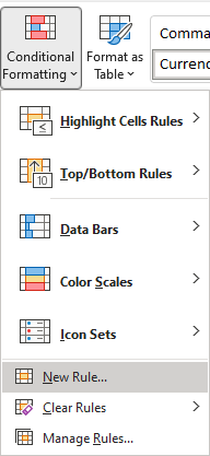
Select the option to Use a formula to determine which cells to format and enter the following:

=ISNA(B1)

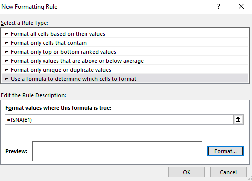
I need to use B1 since that is the start of the range that I have selected. Next, you can just click on the Format button and set the font color to white so that the #N/A values don’t show up. This is what my sheet and chart looks like after applying the formatting:

If you liked this post on How to Hide Zero Values on an Excel Chart, please give this site a like on Facebook and also be sure to check out some of the many templates that we have available for download. You can also follow us on Twitter and YouTube.