Track Warren Buffett’s Portfolio Using Power Query

Billionaire investor Warren Buffett is the CEO of Berkshire Hathaway. And what trades his company is making is always big news among his followers and fans. In this post, I’ll show you how you can use Excel, and specifically Power Query, to determine what the company’s holdings are as of their most recent quarter, and how much they’ve changed over time.

Start with getting the most recent 13f report

Berkshire Hathaway reports its holdings every quarter and you can find those filings on the SEC website. This link filters out the 13f filings for you already. I’m going to click on the Documents button of the most recent report:

On the next page, the key link to use is the html file for the Information Table:

When I click on it, the report itself looks like a convenient table format:

It’s here that you can see the holdings as of the end of the period for Berkshire Hathaway. I’m not going to copy this into Excel but instead, I am going to use the link itself.

Setting up the Power Query link

Back in Excel, I’m going to set up a connection by going to the Data tab and clicking From Web in the Get & Transform Data section. This will prompt me for a URL, where I will enter the link from the SEC website.

Upon clicking OK, the Navigator box shows up, where I have multiple tables to choose from:

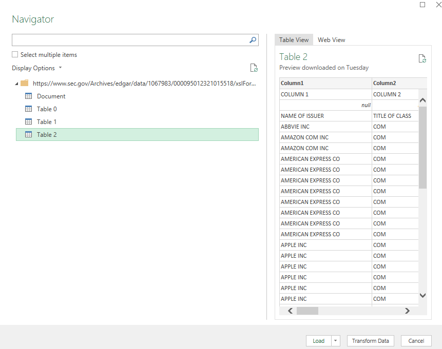
Table 2 is the one that I want as that is the table that has the company names listed and all the other holding details. Since I want to make changes to the data, I’ll click on Transform Data rather than just loading it directly into Excel. Here’s how the table looks:

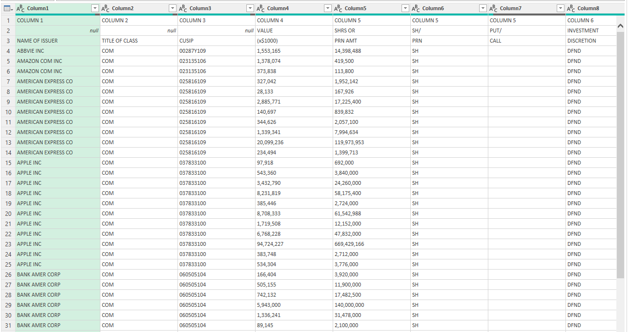
There are a few things right off the bat that I’m going to fix here:

• The headers are not at the top.
• The holdings need to be grouped so that I see the total per company.

To reference the columns easier, it’s important that the headings are correct. First up, I’ll remove the first two rows by clicking on the Remove Rows option in the Home tab in Power Query:

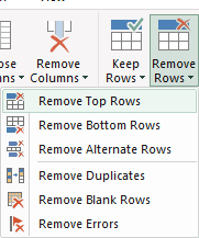
Removing the first two will get the names closer to the top, but the header names remain generic:

To fix this, I’ll click the option to Use First Row as Headers:

Now the first issue is fixed:

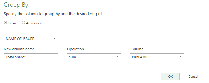
To group the companies, I’ll use the Group By option in Power Query:

On the next screen, I’ll group by issuer (i.e. the name of the company’s shares that are held), set the new column so that it is called ‘Total Shares’, and sum the PRN Amount (shares held):

Now I get a summary of all the shares that are held when grouped by company:

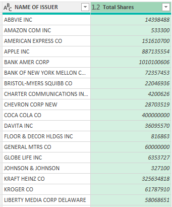
Now I can load this into Excel and have a list of the most recent Berkshire Hathaway holdings.

Comparing to a previous period

Next, I’ll compare the change in position from a previous period. Let’s say I want to go back a year. I can copy this query and just change the source so that it looks at this link from a year ago.

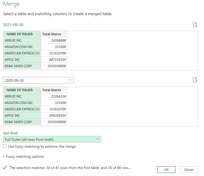
I’ve re-named the queries 2021-09-30 and 2020-09-30 (you can do this simply by right-clicking on the query name). To compare the two periods, what I’m going to do is merge the two queries. In the Merge options, make sure to select a Full Outer join so that all the rows are included. This ensures that you aren’t including just those companies that Berkshire Hathaway still owns shares of.

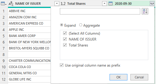
Next, I’ll expand the table to pull in the company name and the shares from the previous report:

This will give me the same values from both tables. One of the things you’ll notice is because of the full outer join, some companies and share values show as null because they don’t exist on both reports:

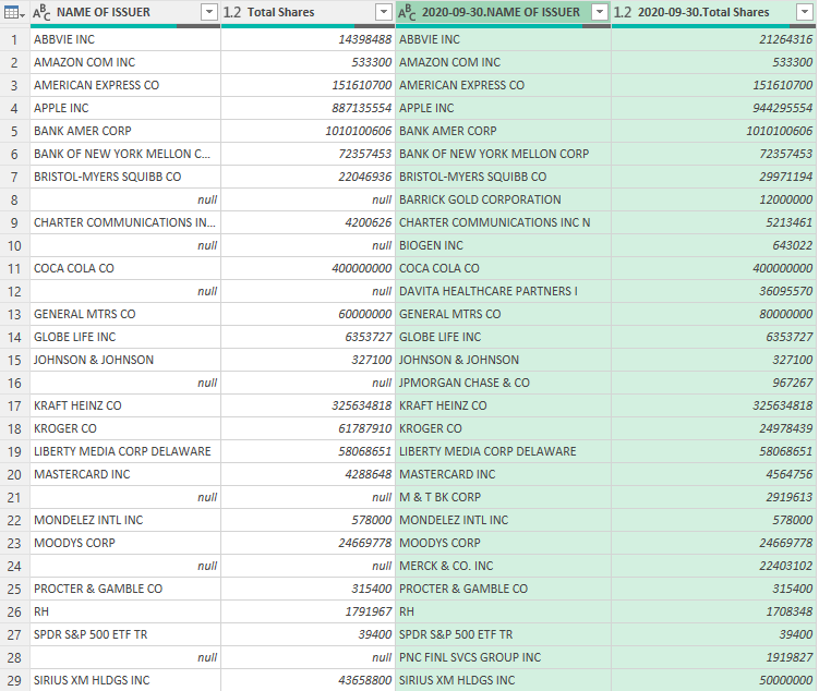
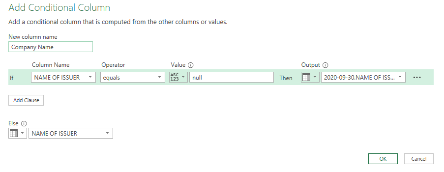
To fix this, I’m going to create a Conditional Column, which you can select from the Add Column tab. The rule I’m going to set up is as follows: if the value in one issuer/name column is null, take the other column’s value. Here’s how it looks:

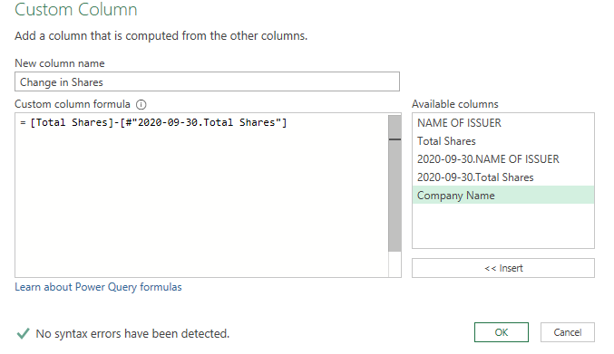
For the change in shares, I’ll need to do a calculation that takes the current holdings and subtracts the previous holdings. But before that, I need to convert the null values where the share numbers are to 0. To do this, select those columns and on the Home tab select the option to Replace Values

Now I can create a Custom Column to calculate the change in shares:

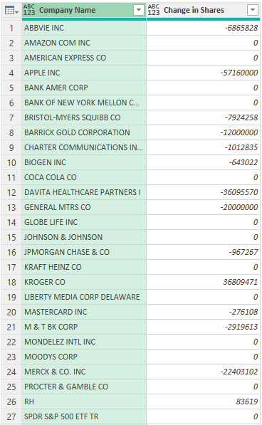
Here’s my updated table after removing the other columns:

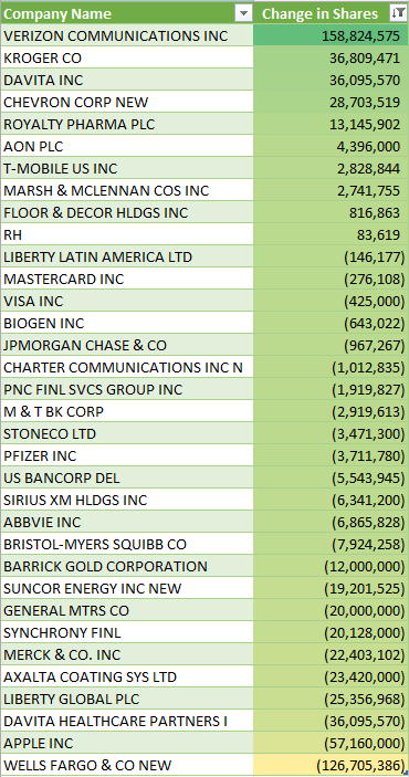
All that’s left is to load the data in Excel. Here’s what the end result looks like after applying some formatting and sorting the values in descending order:

If you liked this post on How to Track Warren Buffett’s Portfolio Using Power Query, please give this site a like on Facebook and also be sure to check out some of the many templates that we have available for download. You can also follow us on Twitter and YouTube.