Inflation has been on the rise and it’s a popular topic these days. In an earlier post, I showed you how to create an inflation calculator to determine what something would have cost in a different year. This time around, I’ll go over how to calculate the actual inflation rate in Excel, showing it as an actual percentage. Let’s get started.
How do you calculate the inflation rate?
If you follow this link to the U.S. Bureau of Labor Statistics, you’ll see a table that has all the latest inflation data. These are indexed values and so to calculate the inflation rate, all you really need to do is take the current index value and divide it by the prior year’s data. For example, September 2022’s inflation rate was 8.2%. To arrive at that, you can simply take the September 2022 index value of 296.808 and divide that by 274.31, which is the value from September 2021. The result is 1.082.
You could download this table into Excel and do a series of lookups to do these calculations. But that’s effectively what I did in the previous post. This time around, I’m going to make this much more automated and involve Power Query.
Download the data using Power Query
First, go to the Data tab in Excel, and click on the From Web button next to Get Data. Then, paste the URL from the link that has the inflation data. Then, you’ll see the Navigator page for Power Query, where you can select from the different tables that are found on the webpage:
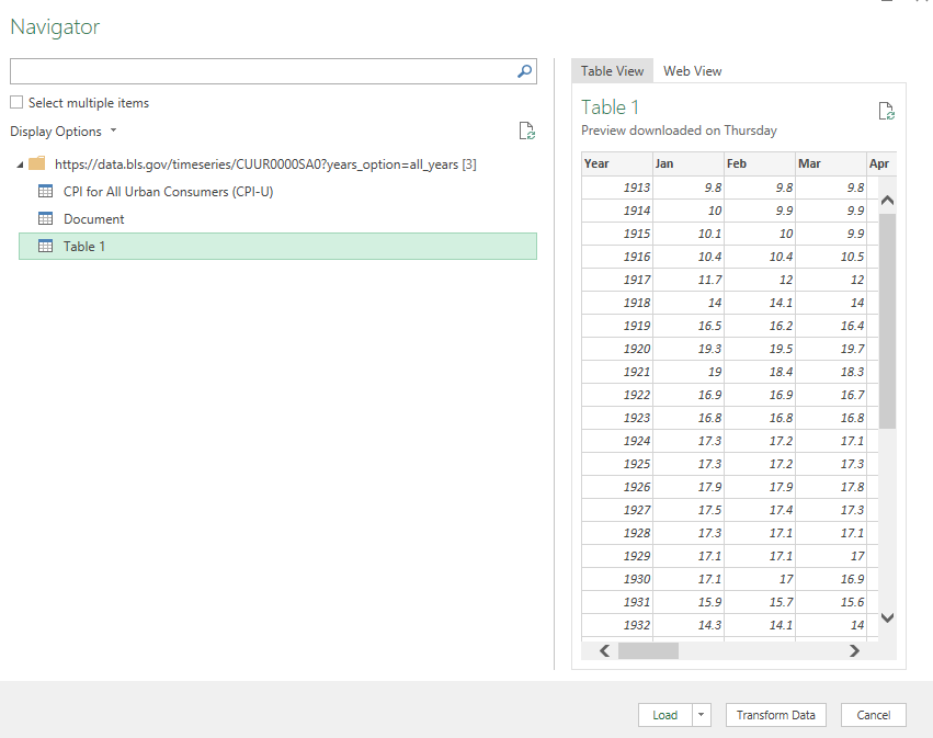
Table 1 is the one that contains the inflation data organized by month and year. Before loading this into my spreadsheet, I’m going to make some adjustments so that I can easily calculate the inflation rate right within Power Query. To do that, click on the Transform Data button.
Modifying the data in Power Query
By default the data shows in the following format:
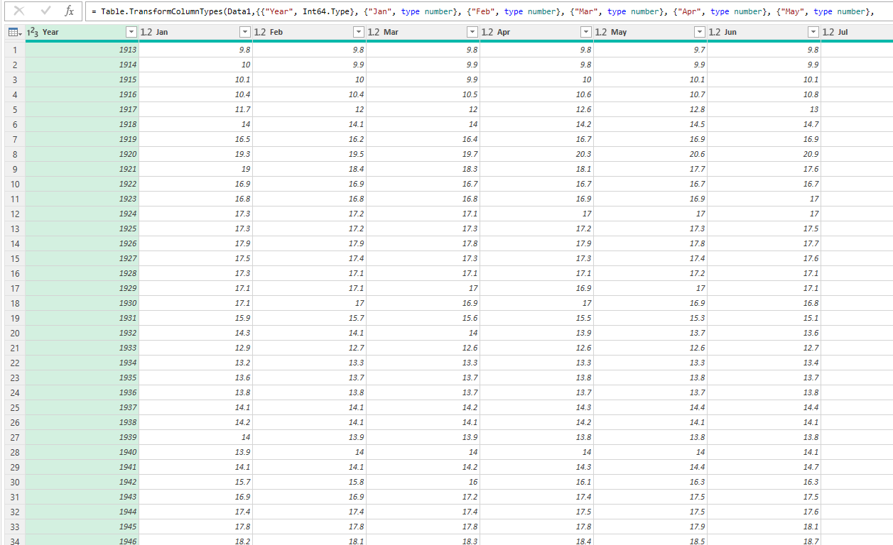
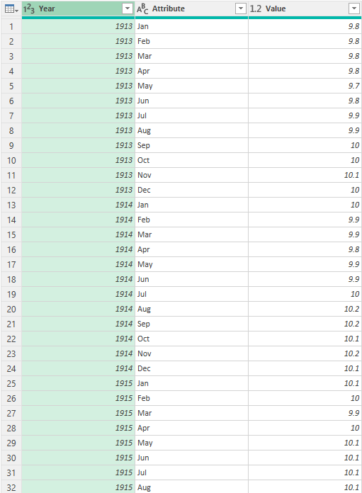
I want the years and months to both be in columns. That means I need to flip the months. To do this, I’ll right-click on the Year header and select Unpivot Other Columns. And then voila, my data is in a more manageable format:
Since I want to compare to the previous year, I’ll also create another column for the previous year. To do this, I can just select the Year column and in the Add Column section, click on the Standard icon that shows different mathematical operators and select Subtract:
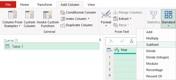
The next screen will ask me for the number I want to subtract from each value, which will just be 1. After entering that and clicking OK, I will have a new field, which I will re-name to PreviousYear.
Next, I’m going to create a combined field for the year and month. First, I’ll convert the Year and PreviousYear fields to text. This can be done by clicking on the icon in their headers and selecting Text.
Then, under the Add Column section, I’m going to select Custom Column. From there, I can enter the following formula to concatenate the fields:
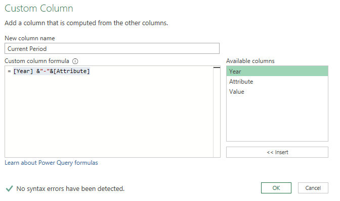
I’m going to repeat these steps for the PreviousYear, and that column I’ll call the Previous Period.
Next, I’m going to split this table into two. I’ll rename the current table to Current. Then, I’m going to create a copy of it by right-clicking and selecting Duplicate, and I’m going to call the new table Previous. In the Current table, I’m only going to leave the following columns: Current Period, Previous Period, and Value. While on the Previous table, I’m only going to include the Current Period and the Value.
What I will do next is to merge the tables, where I’ll be looking up the prior period’s value. To do this, I’ll go to the Current table and under the Home tab, select the option to Merge Queries. I’m going to connect the queries with the Previous Period from the Current table to the Current Period in the Previous table. The goal here is to be looking up the prior-year period:
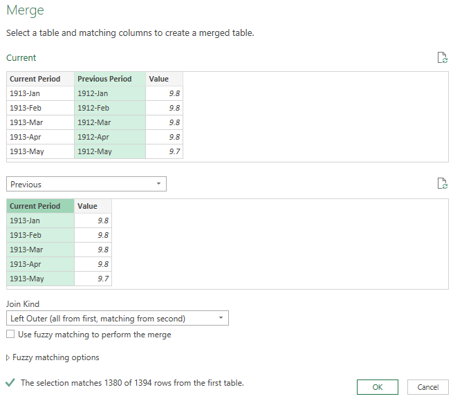
Next, I’ll click on the icon in the newly created column to expand the fields out:
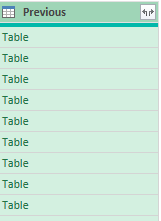
I’m only going to select the Value, as that is the prior value that I want. I’m going to rename that field the Prior-Year Value:
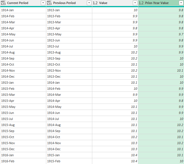
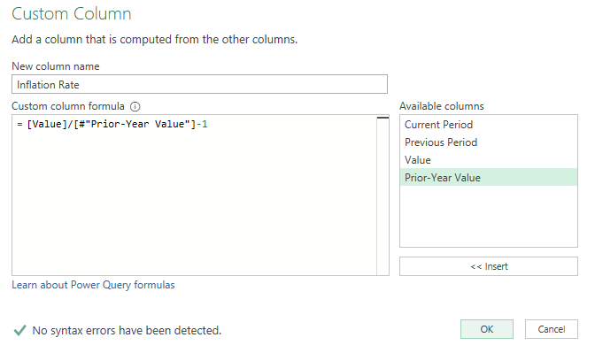
These values shouldn’t be the same and you can easily check to make sure that they are correct. For example, 1914-Jan will show up in both the Current and Previous Periods. And those corresponding values both show 10. Now that I’ve got the current and previous values, the next step is to calculate the percent change. To do this, I’ll create another Custom Column, with this as my calculation:
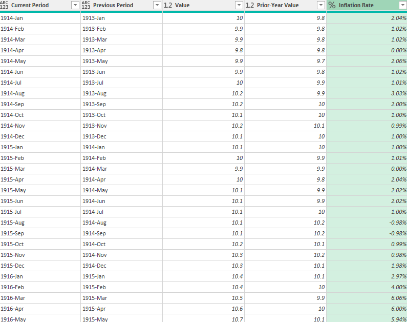
I’ll then convert the field so that it is in a percentage format, and here is what my inflation rate column looks like:
The only thing left at this point is to clean up the Power Query table to remove any unnecessary columns and values. I will filter out any values that are empty. To do this, I’m going to click on the drop down for the Inflation Rate header and select Remove Empty. This will get rid of the values that didn’t have a prior year value. I’ll also remove all the columns except for the Current Period and the Inflation Rate.
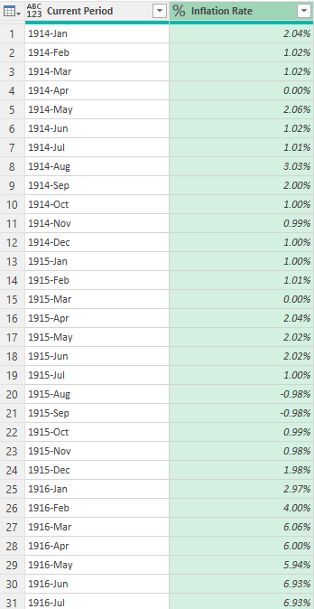
Now that my transformations are complete, I can load this into Excel using the Close & Load button on the Home tab. It will load the Previous table as a new tab, but I can delete that so that I only have the Current table.
Now, moving forward, as the inflation rate data updates, I can just right-click on this table and click Refresh, and Power Query will load the data and calculate the latest inflation rate for me.
If you liked this post on How to Calculate the Inflation Rate in Excel, please give this site a like on Facebook and also be sure to check out some of the many templates that we have available for download. You can also follow us on Twitter and YouTube.

