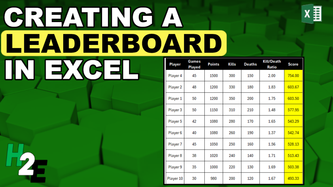
Creating a leaderboard in Excel is a great way to visually rank and compare performance, whether it’s for sales, gaming scores, or any other competitive metrics. Below, I’ll guide you through the process of creating a basic leaderboard in Excel. Here’s a table which shows player scores based on points, kills, and deaths.

Setting up a scoring system
If you just have a single metric for points to sort a leaderboard on, then all you need to do is sort the data. But in more complex situations, you may want to apply weights to calculate a score, which you can then sort. In the above table, there are points, and a kill/death ratio would could be useful in determining a total score.
You may for example, want to multiply the points total by a factor of 0.5 and multiply the kill/death ratio by 2, to get a combined score which considers both metrics. Assuming the points value is in column C and the kill/death ratio is in column F, here is how the formula for the score would look, starting with the first value in the second row:
=C2*0.5+F2*2
By calculating a weighted average, you are effectively creating a tiebreaker in the situation where the points are the same. In this example, Player 1 and Player 2 have the same points. But with a better kill/death ratio for Player 2, that player earns the higher score.

Ranking the top players
The above table isn’t sorted according to score. To sort the leaderboard, all you need to do is to click a value in the score column, and on the Data tab, click on the button to sort the values in order from Largest to Smallest. This now gives us a list that has sorted the players in order of their scores.

To refresh the data, simply click on the sort button again, which will re-sort the data.
Another option to sort the data is by using the SORTBY function. If you’re running the latest version of Excel, you’ll have access to this function. Here’s how you would enter the formula assuming the data is in a table called Table1:
=SORTBY(Table1[Player],Table1[Score],-1)
This returns a single array of data showing the player standings:
The benefit of using this formula is that the data will automatically re-sort the leaderboard for you; there is no need to click a button to sort. Since it is an array function, it will update as you enter updated values.
If you want to return the entire sorted table, you can use the following formula:
=SORTBY(Table1[[Player]:[Score]], Table1[Score], -1)
Here is what the array looks like, with some additional formatting added to it:
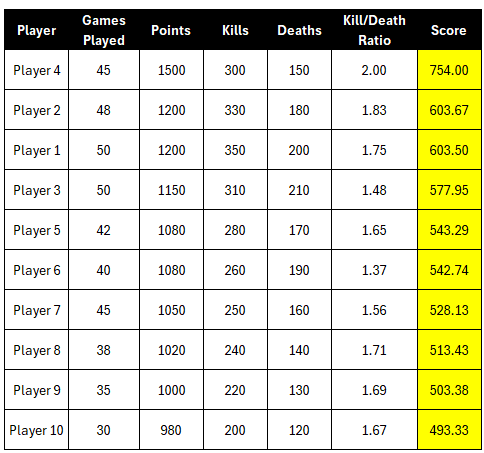
You can add conditional formatting to help identify high-performing players.
If you like this post on How to Create a Leaderboard and Track Standings in Excel please give this site a like on Facebook and also be sure to check out some of the many templates that we have available for download. You can also follow me on Twitter and YouTube. Also, please consider buying me a coffee if you find my website helpful and would like to support it.

