Do you want to be able to use a VLOOKUP with a pivot table? While there isn’t a way to natively do so, there is a way you can make it look as though your pivot table has a lookup function within there, and make it so that it expands along with your data. Suppose you have the following pivot table, which shows employee spending:
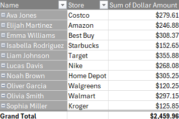
Let’s say we want to look up the department that the employee belongs to, based on the following lookup table:
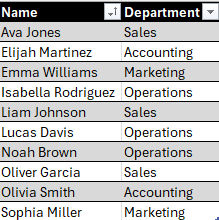
We can’t create a field that does a lookup within a pivot table, but we can make it look as if that’s what we are doing.
Copy your pivot table formatting to make it look as though you’ve added another field
I can create a field called ‘Department’ directly next to my pivot table. And what I can do to make it look as though it’s a continuation of my pivot table is to use the Format Painter so that I can copy the formatting over. To do this, simply select the formatting for the pivot table header, click Format Painter, and then click on the new field. Now it looks as though it’s the same format as your pivot table:
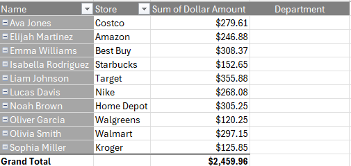
The one drawback is that if you adjust your pivot table, you’ll need to update the formatting. You’ll also want to make sure you don’t expect your pivot table to expand — i.e. you won’t be adding any more fields to expand it horizontally. If you do so, you’ll encounter an error saying that there isn’t enough room for your pivot table. In that case, you can insert a column. But ideally, you would set this additional field once you’ve added all the fields you plan to use in your pivot table.
Using the VLOOKUP function next to your pivot table
The next step is to use the VLOOKUP function the way your normally would. With the employee name in cell A2, and my lookup table in columns F:G, I can set my formula up as follows:
=VLOOKUP(A2,F:G,2,FALSE)
But this is still not ideal as copying this formula down to far will show errors for both grand totals and blank values:
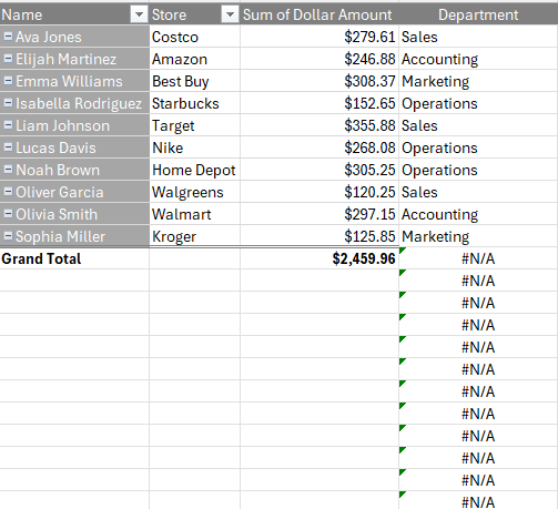
The solution here is to add an IF statement before the VLOOKUP function. In the below example, my formula is checking for both a blank value and a ‘Grand Total’ value. If either criteria is met, it returns a blank:
=IF(OR(A2="",A2="Grand Total"),"",VLOOKUP(A2,F:G,2,FALSE))
Now I can copy my formula down and the formula won’t return a value when the value in column A is blank or is a grand total:
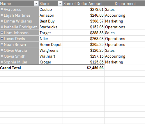
Now it appears as though my lookup function is dynamic and automatically adjusting based on my pivot table selections.
Adding the field to the data set is the ideal solution
Creating a field by adding a formula next to your pivot table can work if your table never expands. But if it might need to, a more versatile option is to simply add the field into your original data set and do the lookup there.
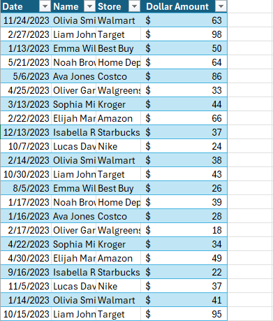
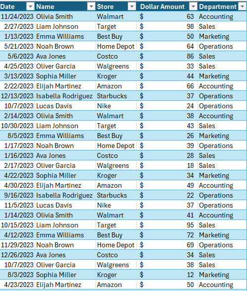
In this data set, I’m missing the department field. But if I add the VLOOKUP formula here, I can pull in the department values right in there. The formula is setup the same and by doing it this way, I can add the field directly to my data set:
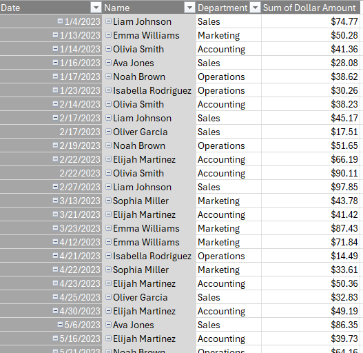
Now, when I update my pivot table I can directly add the department field right into the Rows section:
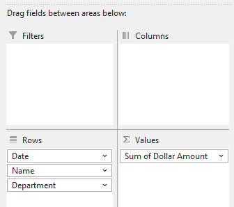
Then, my pivot table shows the additional field, and I won’t run into any issues whether I need to add rows or columns:
In some cases, you might just want a quick way to do a lookup and not adjust the data set, in which case the first method can be preferable. But if you are able to add the field directly into your data set, that is the ideal approach.
If you like this post on How to Use VLOOKUP with Pivot Tables, please give this site a like on Facebook and also be sure to check out some of the many templates that we have available for download. You can also follow me on Twitter and YouTube. Also, please consider buying me a coffee if you find my website helpful and would like to support it.

