Do you have a chart that you want to easily modify the range on, without needing to manually select the data again? Thanks to a new Excel feature, there are now multiple ways you can do that.
1. Creating the chart range as a table
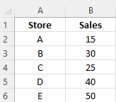
One way you can set up a dynamic chart range in Excel is to put your data into a table. That way, Excel can easily see where you data starts and ends. Suppose you have the following data:
You could show this on a chart but if you needed to add or remove rows from it, your chart wouldn’t automatically re-size. If you deleted data, then there would be gaps on your chart. And if you just added a row, Excel wouldn’t add it to your chart unless you re-selected your range.
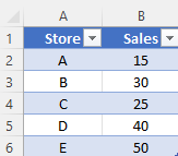
To fix this, you can convert you data into a table. To do this, go to the Insert tab on the ribbon and select Table. You may see some default formatting applied afterwards:
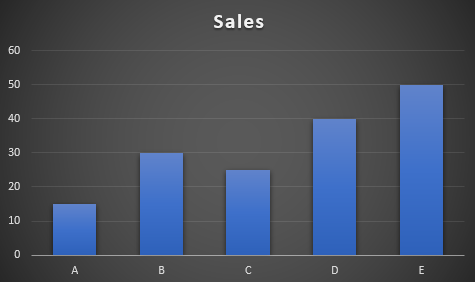
Tables will automatically expand as you add or remove data, and formulas will also copy down by default to any new rows. Currently, this is what my chart looks like for this table:
In the below example, you’ll see data being added and removed from the table, and the change to the corresponding chart.
2. Using an array
If you don’t want to convert you data into a table, Excel has now made it possible to dynamically update your chart using just an array, which is new functionality. From the earlier example, I can create an array that populates the data using the following formula:
=OFFSET(A1,0,0,COUNTA(A:A),2)
The first argument reflects the starting point of the data. The next two are left as zero since I don’t want to actually offset the range. The last two arguments indicate the size of the array, and this is key to making the chart automatically update.
By using the COUNTA function, the formula will automatically adjust based on the number of items in that column. That way, if you add or remove items, the offset function will adjust your range. The last argument (2) indicates that the data set is to two columns wide. Now by updating the source data, both my array will update and so too will the chart:
Arrays are not new to Excel but the ability for them to dynamically update a chart is a new feature. As of now, this feature hasn’t fully rolled out to the public and is only available through the Office Insiders program. To get access to that, you can sign up to be an Insider (free of charge) and then moving forward, you will have Excel’s latest and greatest features as soon as they become available.
If you liked this post on How to Create a Dynamic Chart Range in Excel, please give this site a like on Facebook and also be sure to check out some of the many templates that we have available for download. You can also follow us on Twitter and YouTube.
Excel’s date and time functions make it easy to calculate the difference between two dates. And in this post, I’ll show you how you can calculate age in Excel. This can include a person’s age, or the interval between two dates. You can also break this difference into years, months, days, minutes, and seconds.
Use the YEARFRAC function to calculate the time in terms of fractions of years
One of the easiest ways to calculate age is by using the YEARFRAC function. As the name suggests, it will give you the fraction of a year. Suppose you wanted to calculate the difference between the start of the year 2000 and Christmas 2022. This is what your formula would look like:
=YEARFRAC("1/1/2000","12/25/2022")
Note that depending on your regional settings, you may need to enter date values in different formats. Alternatively, you could simply reference cells that contain date values so that you don’t need to do any hardcoding here.
The above formula will return a value of 22.983. Since Christmas falls towards near the end of the year, the number is close to 23. If instead you choose Jan. 31, 2022 as the end date, then the formula would return a value of 22.083.
Use the TODAY function to make your formula dynamic
To calculate age so that it is always going to be up until today’s date, you can use the TODAY function. This avoids you having to enter the current date each time you want an up-to-date calculation. For example, if you wanted to calculate the fractional years between the start of 2000 and today, your formula would look like this:
=YEARFRAC("1/1/2000",TODAY())
The TODAY value will automatically update so you don’t need to do anything to trigger that calculation. Just by opening your workbook, Excel will pull in the current date value, and your formulas that contain the TODAY function will adjust accordingly.
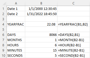
Calculating month, day, hour differences
If you want to calculate the difference in months rather than fractions of years, there’s an easy way you can do that as well. Excel has a DATEDIF function that can make that process quick and easy. The logic is the same as with the earlier formula, but the main difference is that you enter “m” for a third argument, indicating month. Here’s the formula, using the same values as earlier:
=DATEDIF("1/1/2000","1/31/2022","m")
This formula gives a result of 264, which equates to 22 years. You’ll notice the drawback here is there are no fractions or rounding, just 264 months. If I adjust the end date to the start of February (“2/1/2022”), then it will return a value of 265 months. Until the month is complete, the formula won’t add the extra month, even if you’re selecting a date that’s nearly at the end (e.g. January 31).
One alternative you can make is to calculate the difference in days:
=DATEDIF("1/1/2000","1/31/2022","d")
This formula will return a value of 8,066. If you were to divide this by 365, you would get 22.09863. That’s the same answer I would get using the YEARFRAC function if I entered the last (optional) argument in that function to specify that I wanted to use 365 days for my calculation (the default calculation uses 360).
DATEDIF doesn’t have an argument that lets you calculate hours or minutes. However, with the number of days, you can approximate that by multiplying by hours. If you did want to get to that precise level of detail, you would need to create a separate formula for hours and minutes — and you would also need to ensure your date values included that level of detail to avoid approximation.
Using the HOUR, MINUTE, and SECOND functions, you can subtract the starting date from the ending date to arrive at a difference for each of those time calculations.. For these types of details, you should reference the cells as opposed to key in the hour, minute, and second values to ensure everything is entered correctly.
If you liked this post on How to Calculate Age in Excel, please give this site a like on Facebook and also be sure to check out some of the many templates that we have available for download. You can also follow us on Twitter and YouTube.
There are numerous ways to display numbers in your reports. Using percentages and decimals are two common ways to do so. In this post, I’ll cover when it might makes sense to use percentages and when to decimals may be more appropriate. I’ll also provide you with some easy-to-use formulas that will allow you to convert percent to decimal, and vice versa. You can do these calculations whether you’re in Excel or just have a calculator handy.
Converting between percent and decimal
If you want to convert numbers between percent and decimal, the process is incredibly simply in Excel. Select the value(s) you want to change and then select the format you want.
However, if you’re not using Excel, you can still accomplish this manually. To convert a percent into a decimal, all you need to do is to pretend you’re moving the % sign two spots to the left, and then convert it into a period.
In the case of 50% it becomes .50, or 0.50, depending on whether you want to display the 0 in front. This also works with large percentages, such as 1,000%. That’s a significant percent, but the same logic applies, and following the same steps would convert the value to 10. That tells you that the new value is 10 times the size of the original value.
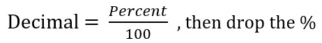
To convert back into percent, you multiply the value by 100 and drop the % sign.
Formula for converting decimal to percent:
Formula for converting percent to decimal:
How to calculate percent of something versus percent change
One important distinction you should consider is to determine whether you’re looking at a portion of something, or a change in value. If you’ve eating half of a pizza, that’s 0.5 of it, or 50% of it. But if you’re talking about the price of something going up by 10%, that’s a slightly different calculation.
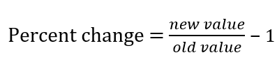
Let’s take the stock price of Microsoft as an example. At the start of 2020, its stock price opened at $158.78. By the end of 2021, it finished the year at $339.32. If we take the ending price and divide by the beginning price (339.32/158.78), then that gives us 2.14, or 214%. It would be correct to say that $339.32 is 2.14 times $158.78. But it would not be correct to say the stock price increased by that amount. That’s because you’re not calculating the actual increase in value. To do that, you need to subtract 1, to arrive at 1.14, or 114%.
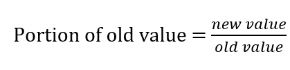
If the stock didn’t increase at all, you would be left with an equation of 158.78/158.78, which would be equal to 1, or 100%. The ending value was 100% of the beginning value, but it certainly wasn’t an increase of 100%. Thus, the need to deduct 1 will give us the correct answer in that case — a 0% change. The same goes for decreases. Suppose the stock fell by 30% to $111.15. Dividing $111.15 by $158.78 would tell you the price is now 70% of the value it was at the start of the year. That’s correct, but to get the percent change, you deduct 1 from that, which tells you it declined by 30%.
The formula for percent change:
The formula to calculate the portion or relative size of something:
It’s a subtle difference but it’s an important one to note, which can prevent you from making a mistake in your calculations.
What to do if your decimals or percentages are very small
If you’re dealing with numbers that go to four or five decimal places, it may not be helpful to display them as percentages or even as decimals. For example, if you were to say the odds of getting struck by lightning in your life were 0.00654% or 0.0000654, whether you use decimal or percent isn’t going to be helpful in conveying those adds.
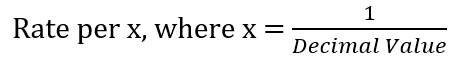
One thing you can do is flip those numbers around by calculating the inverse. By taking 1/0.0000654, that returns a value of approximately 15,300. Stated another way, it tells us that the odds of getting struck by lightning are 1 in 15,300. It’s a far more effective way of communicating the odds as you’re no longer dealing with miniscule percentages that can be hard to visualize.
The formula for converting from a decimal value to a rate:
As you can see from these formulas, they are fairly simple and can be incorporated into your spreadsheet and even done just on a calculator. You could create LAMBDA functions with these formulas, but they involve so few steps that the time savings may not amount to much.
If you liked this post on How to Convert Percent to Decimal, please give this site a like on Facebook and also be sure to check out some of the many templates that we have available for download. You can also follow us on Twitter and YouTube.
Warren Buffett fans like to track the billionaire investor’s moves, and a good way to do that is through Berkshire Hathaway’s 13f filings. His company reports its holdings every quarter, showing where there were changes in its positions. By looking at multiple filings, investors can track the changes from one period to another. With this free template, you can do that quickly and easily all on your own. All you have to do is specify the specific filings that you want to compare to one another.
How the template works
This template uses PowerQuery to grab the data from the 13f filings. It will then compare the two to find the changes in share count.
There are only two inputs you need for the template, both are on the Current.Holdings tab. You’ll need to paste the URL for the current 13f filing and the previous one (or whichever filings you want to compare against one another). It can sometimes be a bit tricky to get exactly what you’re after. Here’s how you can find the 13f filings for Berkshire Hathaway to use in this template:
Do a search for 13f so that you can see just the 13f filings on that page:
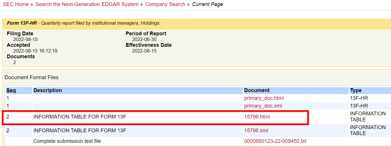
4. Find the reporting period you want and click on the Filing button — don’t click on the actual description next to it.
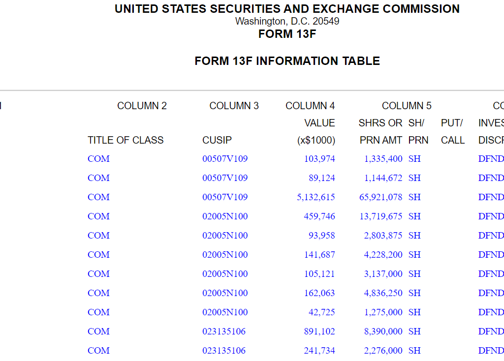
5. When you open up the link, you should see multiple files you can open. Select the information table that is in html format:
When you open the file, you should see the holdings in a table format:
If this is what you see, then the link you’ve downloaded will work. Note, on older 13f filings (e.g. 2013 and older), the format is in a text file and they won’t work with this template.
6. Copy the link and enter it into one of the fields on this template, either for the new filing or the old one.
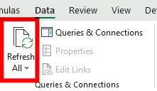
7. Once you’ve filled in both the new and old links, then go to the Data tab in Excel and click on Refresh All. This will update the queries that the template relies on, and calculate the changes.
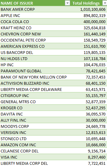
Now the different sheets will update:
Current.Holdings: this will show you the current holdings as per the New13f file
Change.In.Holdings: this will show you the change between the two filings. The change will be reflected in total shares and as a % of change in shares.
Old.Holdings: this will show the number of shares held per the Old13f file.
If you like the Berkshire Hathaway 13f Template, please give this site a like on Facebook and also be sure to check out some of the many templates that we have available for download. You can also follow us on Twitter and YouTube.
Conditional formatting cells can be an effective way to highlight values so that they can easily stand out. You can apply similar logic to charts, and in this post, I’ll show you how you can use conditional formatting with Excel charts. By doing so, you can highlight gaps and key numbers.
Create more than one series to categorize your results
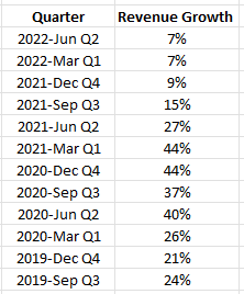
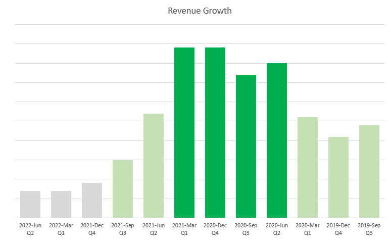
Excel’s conditional formatting isn’t designed to work on charts. But one way you can still achieve the same results is by categorizing results, and creating a series for each category. Here’s an example, using Amazon’s sales growth. Below are the year-over-year growth rates it has achieved over the past 12 quarters:
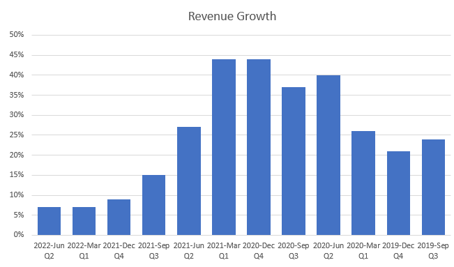
Charting the data out would show the highs and lows effectively:
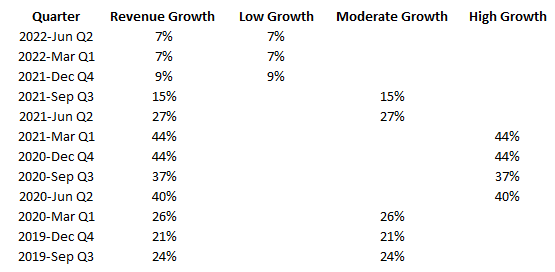
However, suppose you wanted to highlight the high-growth periods (30% or more), with the more moderate ones (15%), and the quarters which were below that. To do that, I’m going to add a few more columns and use IF statements to populate the columns based on the growth rate.
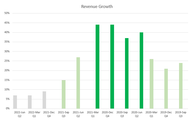
Now, if I populate these values on a chart, they shows up like this:
These column charts are skinnier and that’s because they are taking up more space as there are three different series for each quarter. To get around this, I can just change the charts so that they are stacked. Since only one of these columns will ever contain a value, there’s no danger they will actually ever stack. But by changing the chart type, they won’t take up as much space.
The advantage of this approach is that you don’t even need to rely on the axis to determine what range the growth rate falls within. Although you have to create additional columns by doing this, you can hide any columns that you don’t need to see. You can apply this type of logic to other types of charts as well.
If you like this post on How to Apply Conditional Formatting to a Chart in Excel, please give this site a like on Facebook and also be sure to check out some of the many templates that we have available for download. You can also follow us on Twitter and YouTube.
Switching back between Celsius and Fahrenheit can be cumbersome if you haven’t memorized the formula. There are multiple steps involved and you can easily make a mistake. And while you could use shortcuts to try and approximate roughly how it is, you can be more precise if you create a formula that you can use over and over again. If you’re using Excel, you can save yourself a lot of time as you can convert from Celsius to Fahrenheit (as well as in the other direction) using a formula which can compute the results in an instant.
What the formulas look like
The formula to convert from Fahrenheit to Celsius is as follows:
C = 5/9 x (F-32)
And this is the formula for the reverse:
F = (C x 9/5) + 32
You could set these formulas up in Excel just with simple arithmetic. The downside of that is then you have to create multiple formulas (one for Celsius and one for Fahrenheit), or even set up a small template just to do that. But Excel makes it even easier do to that as it has a function which can save you all those steps — it even knows the formula so you don’t have to memorize it!
Using the CONVERT Function
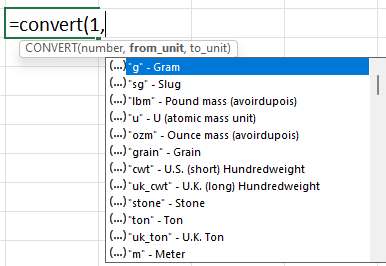
There’s convenient function right within Excel that can convert between different measurement values, called CONVERT. As the name suggests, it can convert values for you. It takes three inputs: the current value, what unit you’re converting from, and the unit you want to convert to. The formula to convert Fahrenheit into Celsius is as follows:
=CONVERT(A1,”F”,”C”)
Where A1 is the value in Fahrenheit. To do the reverse, you just need to flip the symbols:
=CONVERT(A1,”C”,”F”)
The key thing you just have to remember is that the unit you’re converting from comes first, followed by the unit you’re converting to. Those values need to be in quotes so that Excel reads them correctly as a text values.
This function is a lot more powerful and there are even more items you can convert between, simply look through the list of possibilities as you are entering the arguments.
You can flip between date values, measurements, weights, and many other things. The CONVERT function is much more powerful and converting between Celsius and Fahrenheit is just one of the many things it can do.
If you like this post on How to Convert Celsius to Fahrenheit Using an Excel Formula, please give this site a like on Facebook and also be sure to check out some of the many templates that we have available for download. You can also follow us on Twitter and YouTube.
The Annual Percentage Rate (APR) on a loan tells you what your total borrowing cost is per year. It’s different from just the interest rate because it will include other expenses and fees relating to a loan. And for that reason, the APR will be higher than the interest rate. If there are no additional fees, then it will be the same. In this post, I’ll show you how you can calculate APR in Excel and how it compares with just the interest rate itself.
Functions used to calculate APR in Excel
In order to calculate APR in Excel, there’s a simple function that can allow you to do that quickly and easily; there’s no need to draw out and complicated formulas for APR that you might find online. The key is to just determine your inputs and the variables you will be using for the calculation.
The RATE function in Excel will take care of the calculation but it requires the following inputs:
Number of periods
Payment amount
Present value
Future value
The only one of these that may require some additional work is the payment amount. However, there’s also a function for that too, called PMT.
Calculating APR using an example
I’ll illustrate how you can calculate APR in Excel by using an example. Suppose you’re taking out a loan for $200,000 where you’ll incur financing fees of $30,000. The interest rate will be 4% and term is 10 years. And payments are made on a monthly basis.
For starters, we need to calculate the monthly payment amount. That requires similar inputs to the RATE function except instead of a payment amount, we need the interest rate. And since payments are going to be made on a monthly basis, both the interest rate and the term needs to be expressed in months. Instead of 4%, the rate we’ll need to use is 4%/12 and the term will be 120 months.
The PMT formula will look as follows:
=PMT(0.04/12,120,-200000,0)
Instead of entering in the interest rate to the decimal point, I’ve left it is a fraction so that the calculation is more precise. The present value is entered as a negative since the 200,000 is what is currently owed, while the future value (0) is what it will be when the loan is paid off.
The result of this calculation results in a monthly payment amount of $2,024.90.
In this scenario, there are no finance charges included. To factor those in, simply change the present value to -230,000. By doing that, you’ll arrive at a monthly payment amount of $2,328.64.
Using those payment amounts, we can now calculate the APR, using the RATE function:
=RATE(120,2024.9,-200000,0)*12
The result of this formula is multiplied by 12 to get to annual rate. This is because the RATE function gives you the rate per individual period. At the monthly payment of $2,204.90 (i.e. when there are no financing charges), the formula for APR results in a value of 4%, which is equivalent to the interest rate. Since there are no additional fees here, it makes sense that the percentages are the same.
However, when using the higher payment amount for the loan that includes finance charges, there will be a more noticeable difference. For that calculation, the formula is as follows:
=RATE(120,2328.64,-200000,0)*12
What you’ll notice here is that while the payment amount has changed, the loan remains the same. This is because while we need to pay for the extra finance charges and they are added to the monthly payment, the value we would be receiving remains just $200,000. Through this calculation, we arrive at an APR of 7.06%.
The higher the additional fees and charges, the bigger the delta will be between the APR and the interest rate.
Creating the amortization tables
The differences in these rates can also be demonstrated through an amortization table to show how the loan is paid off. For an amortization table, we need the following fields:
Payment #
Beginning Balance
Principal Payment
Interest Expense
Ending Balance
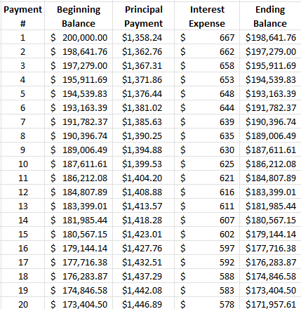
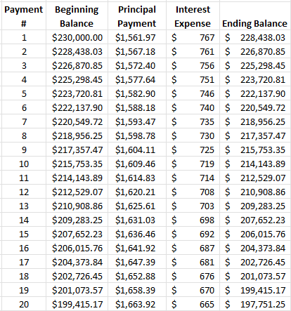
The beginning balance will be the total that needs to be paid off. The interest expense is the calculated by taking the balance and multiplying it by the interest rate. What’s left over from the monthly payment goes towards the principal. How much is paid off is reduced from the beginning balance to arrive at the ending balance. Here’s how the table will look in the first scenario, where there were no additional finance charges:
This excerpt shows the first 20 payments. The following is the amortization table for the second scenario, where finance charges total $30,000:
Here you can see that with a higher balance, more of the payments are going towards interest at the start. Although it takes the same amount of time to pay off the loan, higher payments are necessary to account for the increase in the beginning loan amount.
If you like this post on How to Calculate APR in Excel, please give this site a like on Facebook and also be sure to check out some of the many templates that we have available for download. You can also follow us on Twitter and YouTube.
Nested IF statements aren’t always the most efficient way to structure your formulas. And they can make it difficult later on if you need to fix a formula or make a change to it. What’s worse, is if you inherit someone’s spreadsheet and try to dissect their nested IF functions. In this post, I’ll show you how you can get around using nested IF statements and the different alternatives you can use.
How nested IF statements works
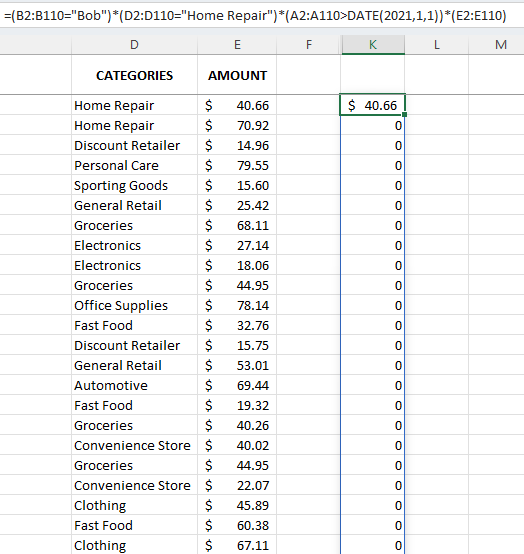
To start, let’s look at how you might construct nested IF statements. Here’s a data set that has different cardholders and their related expenses:
I’m going to create a column with a series of IF statements to see how much Bob spent on home repair since the start of 2021. With a nested IF statement, I might first check if the cardholder is Bob. Then, if that’s true, check if the category is Home Repair. And then, check if the date is after Jan 1, 2021. Here’s how that would look inside of a formula:
You can see this starts to get pretty messy. And the IF statements could continue going on if you have even more criteria you want to fit into here. If I were to copy this formula down, I could get a total of all the values where Bob spent money on Home Repair. However, this wouldn’t be terribly efficient.
You could use a pivot table to quickly summarize the data by cardholder spending and category. But for this example, let’s assume that you need to do it within a formula and can’t rely on creating a pivot table when doing these types of calculations.
Using the AND function to group multiple criteria
An effective option in making your nested IF functions shorter is by using the AND function. It allows you to put all your conditions in one neat formula that you can embed within an IF function. Within the AND function, I can enter all these arguments:
AND(B2="Bob",D2="Home Repair",A2>DATE(2021,1,1))
You can keep on adding to conditions to the AND function for as many rules as you’d like to apply. This can make it cleaner to see all your criteria. All of the criteria within the AND function need to be met for the formula to return a TRUE value. Similarly, you can use the OR function if you want to check if any criteria are met.
The above formula can easily be embedded within the IF function as follows:
This does the same job as the nested IF formula except it’s a lot cleaner. However, the drawback here is that like with the nested IF statement, if you wanted to calculate all of the instances where Bob spent money on Home Repair, you would need an extra column and ad all the values up. That’s still not very efficient.
Using an Array function
Another option you can use for quickly tabulating these results is by using an array function. This can apply the logic to every cell and calculate the total for you. Rather than IF and AND statements, you can evaluate each argument, force a 1 or 0, and then multiply that by the amount to arrive at a total. Here’s how that formula might look:
This formula extends to the bottom of my data set. How it works is that each group of parentheses represents an argument. If it evaluates to TRUE (i.e. the criteria is met) then the value becomes a 1. If the criteria is not met, then it evaluates to a 0. So if all the criteria is met, the results will be 1*1*1 multiplied by the amount in column E. If any one of the conditions is not met, then the result will be a 0. This is the same method as the earlier examples.
The downside of an array is that it will automatically extend to the bottom of the data set:
This again runs into a similar limitation where your formula of using up more cells than you might want to occupy. But to get around this, you could add the SUM function before your array formula:
Another function that can do the job is SUMPRODUCT. With this function, it can take care of all the criteria while also summing up the total in just one cell. The logic is similar to how the array formula was calculated above. The key difference here is to put that all within the SUMPRODUCT function. Here’s how it looks:
This will obtain the same result as if you were using the array function. SUMPRODUCT is used for multiplying arrays but it can be made to work in this fashion as well. The key is making sure you encompass all the arguments withing parentheses (hence why I opened and closed SUMPRODUCT with not one but two parentheses.
As you can see, there are many different ways you can make your formulas more efficient in Excel without having to rely on nested IF functions.
If you like this post on How to Avoid Using Nested IF Statements in Excel, please give this site a like on Facebook and also be sure to check out some of the many templates that we have available for download. You can also follow us on Twitter and YouTube.
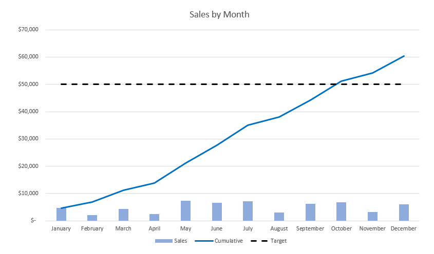
Are you creating a chart that shows progress, with a certain goal in mind? In this post, I’ll show you how to create a chart with a target line so that you can see how close you are progressing toward your goal.
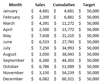
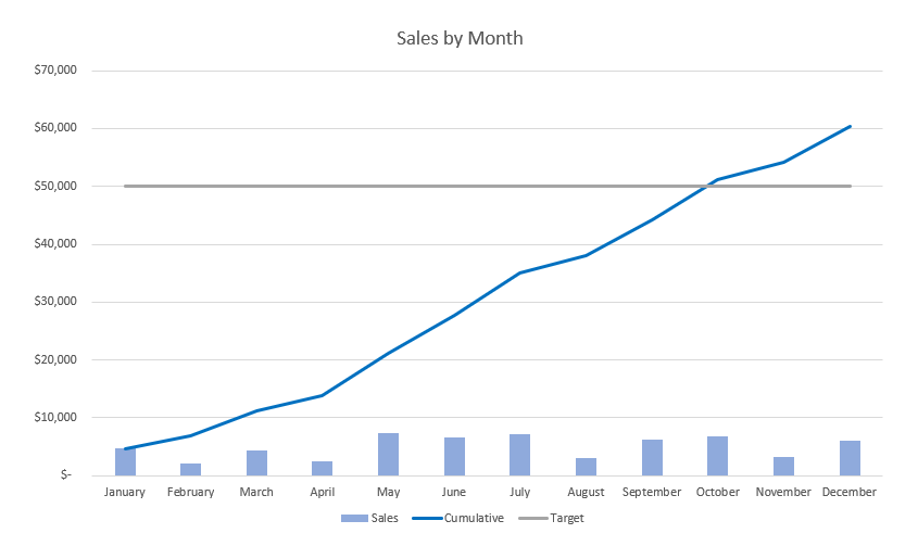
A common example for this type of chart is where you are reporting monthly sales and have a goal you want to reach for the year. Here’s a chart that shows the monthly revenue and has a cumulative total as well:
Creating the target line
To create a target line, I need to add another series to this chart. For example, let’s say your goal is for sales to hit $50,000 for the year. To do that, you just need to create another series. I’ll call it ‘Target’ and for each of the values, I’ll enter in $50,000:
You don’t need to enter $50,000 manually into each cell. You could use the autofill to copy the values down. However, a more flexible way to do this is to enter $50,000 into the first cell, and use a formula to refer to that cell. That way, if you change your target amount, you only need to make the change in one cell.
If you’ve already created your chart and want to add the line to your chart, you’ll need to right-click on the chart and click Select Data. Then, adjust your chart range so that it includes the extra column, and then you’ll see your chart update with the line. If you are creating a chart from scratch, then you just have to select the correct range when first creating it.
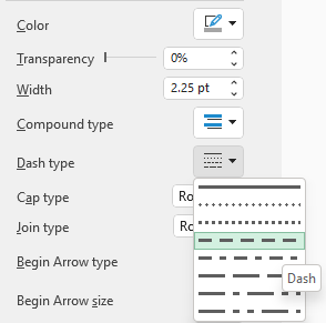
One additional thing you may want to do at this stage is to adjust the formatting of the target line. A good idea can be to make it look different from the other lines on your chart. One way you can do this is by using dashes. If you click on the target line, you will see a pane show up on the right-hand side showing you options to format the data series. Click on the paint bucket icon and you’ll see various settings for the line. There is one option for the Dash type which will allow you to show the line as breaking up as opposed to being solid:
After also changing the color to a solid black, this is what my chart looks like with these changes:
If you like this post on How to Create a Chart With a Target Line, please give this site a like on Facebook and also be sure to check out some of the many templates that we have available for download. You can also follow us on Twitter and YouTube.
You can add lots of automation to your spreadsheet by utilizing visual basic (VBA) and running macros. One of the more common macros you might run include loops. In particular, using for loops in VBA can allow you to cycle through a range of data, check for criteria, and then execute commands. Or, you can also use it to do calculations and to compute totals. There’s a lot of potential with running loops in VBA. In this post, I’ll show you how you can get started with them.
Looping through data in Excel to highlight blank or incomplete data
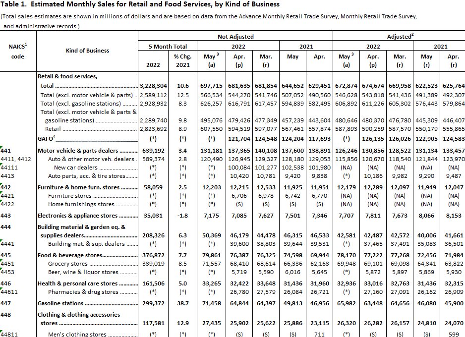
In the following data set, I have some missing values where there is an (*) in place of a value in column D:
I’m going to loop through the column that shows the change value and I will look for the (*) values.
To get started, launch VBA from the developer tab or hit ALT+F11. Then, insert a new module. I’m going to call this subprocedure ‘cleanup’. I’ll start with declaring variables for the worksheet, individual cell I’m looping through, an integer to track how far along I am in the range, and an integer for the last cell within the range.
Sub cleanup()

Dim ws As Worksheet
Dim cl As Range
Dim lastcell As Integer
Dim i As Integer

Set ws = ActiveSheet
lastcell = ws.Range("A1").SpecialCells(xlCellTypeLastCell).Row


End Sub
In the above code, I’ve assigned the worksheet variable to the sheet that I’m on. And I set the lastcell variable to the last row in the sheet. This is the same as if you were press F5->Special->Last Cell. This makes it easy to determine where the data set ends, and gives me an endpoint for my loop. There are other types of loops you can use where you don’t need to specify an end. But this reduces the risk of you getting into a never-ending loop.
As for the loop itself, it will look like this:
For i = 1 To lastcell

    Set cl = ws.Range("D" & i)

        If cl = "(*)" Then

            cl.EntireRow.Interior.Color = vbRed


        End If


Next i
How it works is it uses the i variable to start from 1 and go all the way until the lastcell variable. In this example, that relates to 92 (the last row in my data set).
Then, it assigns the cl variable to each cell in column D as I go through that range. In the first instance, the cl variable is D1, then D2, and so on, until you reach the end (D92).
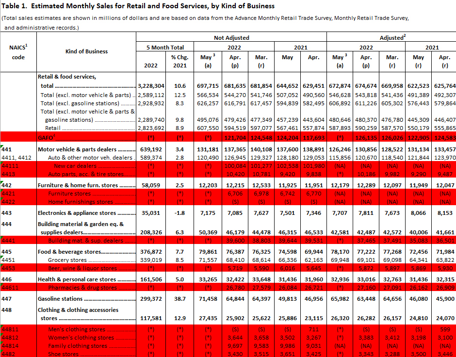
Next, it evaluates if the value of that cell is (*). If it is, then it highlights the entire row in the color red. If I run this macro, this is what my sheet looks like afterwards:
It did the job well, as you’ll notice everything that had a value of (*) in column D, the entire row ended up getting highlighted in red. There are other colors you can use and other things you could have done. Next, I’ll show you how you can just delete these rows entirely.
Deleting rows while looping through data in Excel
Removing rows seems simple enough, but it is a little tricky here. For instance, to remove the row rather than to just highlight it, that involves a simple line of code (in my example I’m referring to my cl variable):
cl.EntireRow.Delete
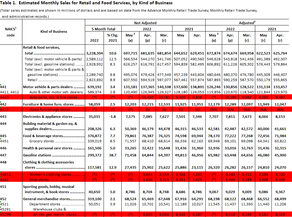
If I run the macro with that code, this is what happens to my worksheet:
I’ve left the red highlighting in place to show you that there are still many rows that should have been deleted and that weren’t. So did the macro simply not work?
The problem lies with how it was set up. In the current macro, I’m moving down from one row to the next. If I’m at row 10 and delete it, then the next row I move on to is row 11. However, the issue is that once I delete row 10, everything moves up a spot. So what was previously row 11 now becomes row 10, causing me to effectively skip over that row and miss it. Now my macro no longer evaluates it.
There are a couple of ways to fix this. One can be that if I delete the row, I can adjust my i variable so that it deducts one so as not to skip over the next row. Just by adding a line of code, you can adjust for that issue:
For i = 1 To lastcell

    Set cl = ws.Range("D" & i)

        If cl = "(*)" Then

            cl.EntireRow.Delete
            i = i - 1


        End If


Next i
The i = i -1 line of code will reset the i variable back down a spot when a row is deleted. This will now prevent the macro from jumping over a row.
However, there’s another option you can use, and that’s looping through the data in the opposite direction.
Looping through the data backwards and utilizing the step keyword
In the first example, I looped through the data from row 1 to the last row. Here’s my full code for that:
Sub cleanup()

Dim ws As Worksheet
Dim cl As Range
Dim lastcell As Integer
Dim i As Integer

Set ws = ActiveSheet
lastcell = ws.Range("A1").SpecialCells(xlCellTypeLastCell).Row

For i = 1 To lastcell

    Set cl = ws.Range("D" & i)

        If cl = "(*)" Then

            cl.EntireRow.Delete


        End If


Next i


End Sub
I’m going to adjust this and go in reverse order. However, it’s not as simple as specifying start from the bottom number and go to row 1. You need to give VBA a bit more information. This is where you can use the Step keyword. By using that, you can specify in which direction you want the loop to go, and whether it should go 1 row at a time or jump multiple rows.
Here’s how the loop looks like if I want VBA to jump backwards one row at a time from the bottom:
For i = lastcell To 1 Step -1


    Set cl = ws.Range("D" & i)

        If cl = "(*)" Then

            cl.EntireRow.Delete


        End If


Next i
If you want to jump by 5 rows, you would use Step -5. However, because I want to evaluate each row, -1 is what I’ll use in this example. By running this loop, now the highlighted rows are all deleted:
Since the loop is starting from the bottom and working its way up, it doesn’t matter that I’m deleting rows; it doesn’t impact the rows above and so no adjustment to the i variable is necessary.
If you like this post on How to Create For Loops in VBA, please give this site a like on Facebook and also be sure to check out some of the many templates that we have available for download. You can also follow us on Twitter and YouTube.