This post will show you how to create the effect of highlighting alternating rows, which sometimes makes it easier to read a data set.
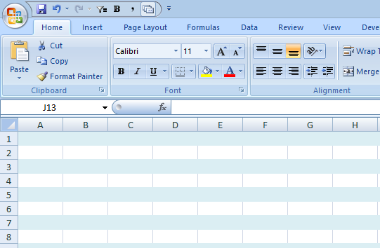
In order to accomplish this, first select all the cells in the worksheet and then select New Rule under conditional formatting.

For the new rule you will need to select the last option to use a formula. The formula we will need to use is as follows:
=MOD(ROW(A1),2)=1
The MOD function calculates the remainder after division and has two arguments, the number to be divided into, and by what number.
Using ROW(A1) means the reference will change depending on the location of the cell, meaning it will encompass every row in the selection. Using 2 as the divisor will help identify if the row is as odd number or even. If you’d rather highlight columns than rows, use the COLUMN function.
The formula will be true if the remainder is 1, meaning the row is an odd number (e.g. highlighting will start on the first row). If you want highlighting to start from row 2, just change the 1 to a 0, since even rows will have no remainder.
Once the formula is set, click on Format to determine the appearance of the alternating rows.

I select a light blue colour for the alternating rows

After I press OK this is the result of my conditional formatting:
If you don’t want to apply the formatting to all the cells or want to change the range, under conditional formatting select manage rules

There you will see a field where the formatting Applies to. Here you can change the range you want the formatting to apply to.