copy paste ctrl c v

How to Copy and Paste in Excel (5 Different Ways)

Knowing how to copy and paste is one of the most basic things you can learn to do in Excel. And while everyone is familiar with doing it, you might be surprised that there are several ways to do it, some more common than others.

Using Ctrl + C and Ctrl + V

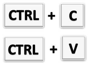
copy paste ctrl c v

This is definitely one of the more common ways that people are familiar with copying and pasting. It simply involves selecting the cells you want to copy, pressing Ctrl + C, and then selecting where you want to paste them, and then clicking Ctrl+ V.

Using the mouse to right-click copy and paste

right click mouse

Also another one of the more common ways to copy and paste. Here you’ll select what you want to copy, right-click and select copy. Then, select where you want to paste the data, then click right-click and paste. This way avoids having to use the keyboard but requires pulling up the menu with two mouse clicks.

Using the mouse and keyboard together

ctrl mouse copy and paste

Hold down Ctrl while selecting the cell that you want to copy and drag it to your destination. Then, release the mouse button and your data will be copied.

Note, if you release the Ctrl button first, and then release the mouse button, then you will have moved the cell (the equivalent of Ctrl + X, Ctrl+V) instead of copying it. The advantage of this method is you don’t have to click as much and it’s useful if you’re quickly copying within the same area. The disadvantage is this method won’t work if you want to copy the data onto another tab or workbook.

Using right-click to copy and paste

right click copy

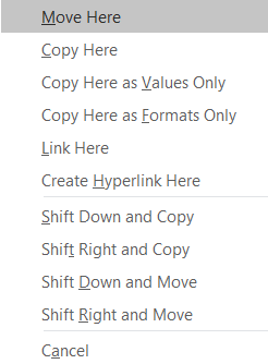
Select a cell and hover over the borders until you see a crosshair appear. Then hold down on right click and drag it to where you want to copy it to, then release the button. You’ll be left with many options, including copying the cell or moving it. Technically this involves a second click, but you only have to bring up the menu once.

right click copy paste menu

Using VBA

This is obviously not a method I’d suggest if you wanted to just copy cells over one time unless it was part of a larger macro you’re working on. But to copy data over in VBA it’s a fairly straightforward process that includes just one line of code:

Range(“A1”).copy Range(“A2”)

The first range (A1) is the cell you’re copying and in the above example, A2 is where you’re pasting it to.


If you liked this post on How to Copy and Paste in Excel (5 Different Ways), please give this site a like on Facebook and also be sure to check out some of the many templates that we have available for download. You can also follow us on Twitter and YouTube.

pivottables4a

4 Biggest Annoyances of Pivot Tables and How to Fix Them

Pivot Tables are great tools, especially for quickly summarizing data and allowing you to avoid entering in complex formulas to do so. However, they aren’t perfect and definitely have their quirks about them.

Here are four things that most users aren’t crazy about, and how to fix them.

The layout

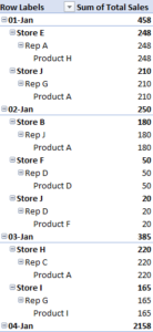
When you create a pivot table it puts the table into a layout that is less than optional for spreadsheets. It’s not only hard to use for any other purpose, but it’s also not the easiest format to read. I always prefer a format that resembles more of a spreadsheet itself, in a grid format, without the indented rows.

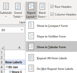
To change the format, go to the Design section of the PivotTable Tools and select Report Layout and select Show in Tabular Form

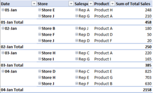
This is what the pivot table looks like after the change:

This might still look a little cluttered, but what you can also do is get rid of any subtotals by simply right-clicking on the Total and unchecking the Subtotal button, and then it’s a bit cleaner:

The table still needs a little work for me, and that brings me to the second issue:

Labels do not repeat

You’ll notice that the value in the date field only shows up once. And so if I had many entries for a given date there would be a lot of blank values in the first column. Again, this is not ideal for a large data set and so this is where I’d like to make a change as well.
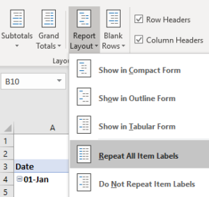
I go back to the Report Layout section, except this time I select the option to Repeat All Item Labels

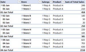
Now my table looks like this:

This is what I would hope the pivot table looks like right off the bat. Unfortunately, Microsoft does not agree and opts for the indented version with subtotal at every section and no repeating values.

But that’s not all, there’s another little nuance you may notice when it comes to pivot tables:

Formatting won’t stay consistent

You’ll notice that in the sales data, I have a total of 2158 for January 4th. Anytime you’re dealing with numbers in the thousands, you’ll probably want some formatting that shows a comma in there just to make the numbers more readable. However, if you simply select the entire column and change the formatting, it will revert back to the default if you refresh the pivot table after adding more data.

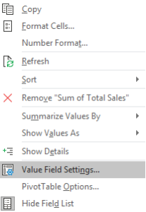
What you need to do is actually change the field settings. To do this, right click on any of the numbers in that column and select Value Field Settings.

From there, select Number Format and then select the format you want it to show up as. Doing this will ensure the formatting won’t change when you refresh the data.

Tip: if you routinely make these changes like I do, you may want to check out the add-in I created which will make all these changes for you at the click of a button.

This brings me to the fourth most irritating item when it comes to pivot tables:

GETPIVOTDATA

By default, when you reference a number in a pivot table, it will auto-generate a formula called GETPIVOTDATA. In most cases, you probably won’t find this helpful, especially if you just want to reference some pivot table values elsewhere in your workbook. If you just want to reference cell E4 and copy the formula down, you’ll need to adjust the pivot table settings, as the GETPIVOTDATA will make it a bit painful to accomplish this.

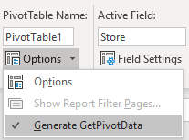
Back under the PivotTable Tools section, select the Analyze tab and on the Options menu on the left-hand side, uncheck where it says Generate GetPivotData

Now you can reference values from a pivot table the way you would any other cell in your workbook.

If you have any other frustrations with pivot tables, please share them in the comments.

stacked1

Using Stacked Charts and Showing Totals


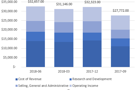
A stacked chart in Excel allows users to take advantage of the best of both worlds: a column chart that shows period-over-period totals and a pie chart that can show what made up those totals. It can be a very useful chart, but knowing how to structure it is half the battle.

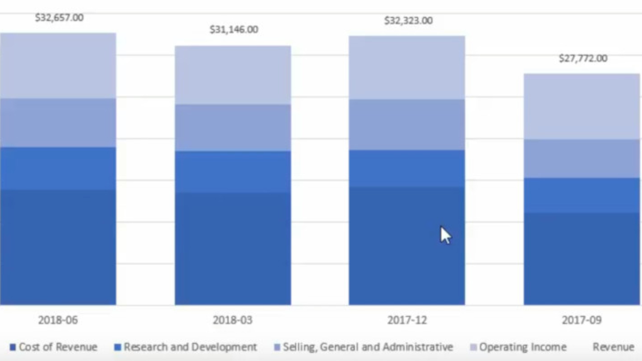
In my example, I pulled Alphabet’s earnings for the most recent four quarters. I wanted to show a) the period-over-period sales as well as where those sales went, and how much flowed through to the company’s operating income.

Below is the table that I used:

The key things is you want to make sure that all your categories add up to the amount that you’re trying to reconcile (in my case, it’s revenue).

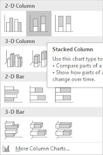
Once the data is ready, select the data and insert a Stacked Column

stacked column chart excel
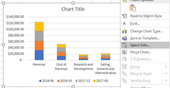
In my example, the categories showed on the horizontal axis, which is not what I wanted, so in order to fix that, right click on the chart and press Select Data
stacked column chart excel
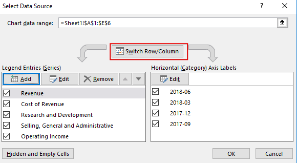
From there, you want to hit the button to switch row/column:
chart switch row and column excel
This will give you a stacked chart. The problem, however, is that my total (revenue) is mixed into this, and that’s not going to give me the desired result. After all, I want to see where the revenue goes, not include the revenue in my categories.
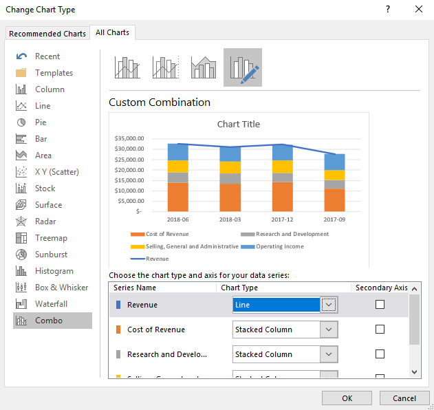
To fix this, you’ll want to right click on one of your column charts and select Change Series Chart Type

excel change series chart type

That should take you to the Combo section. If it doesn’t, make sure to select it. All your series should show a stacked chart. You’ll want to change the revenue series to a Line chart. By doing so, it will not contribute to the stacked chart and now it’ll simply be made up of the other categories. 
combo chart excel
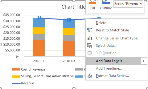
Next, add data labels for the line chart so now you’ll see the totals. To do this, right click on the line chart and click Add Data Labels


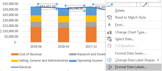
The problem is the labels show to the right, and it probably makes more sense for these labels to show above the stacked chart. Right click on any of the labels and select Format Data Labels

excel chart format data labels

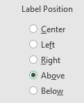
Make sure that for the label position, Above is selected
excel chart format data labels
Now my chart is starting to come together:
excel stacked line chart
Except I still have that line going over the top of the stacked charts. To get rid of the line, right click on the line chart and select Format Data Series

excel chart format data series

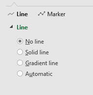
Select No line from the Line section
excel chart format line

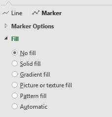
Now, select the Marker and make sure the fill option is set to No Fill
excel chart format marker
Now, I’ve gotten rid of the line completely:
excel stacked chart
At this point it just comes down to designing the chart how you want it. Some of the changes I made included:
  • Getting rid of ‘Revenue’ from the legend
  • Changing the color theme
  • Shrinking the gaps between the stacked charts
excel stacked chart
error1

Formatting and Removing Errors and Zero Values

Often times in a data set you’ll have to handle with errors that can wreck your data, especially if you need to do any analysis on it. There are several ways that you can handle errors so that they don’t show up in your data.

IFERROR

The first method is by using the IFERROR function, which allows you to easily replace the error with whatever you want in its place. If you want a numerical value, you may want to put in a 0, otherwise you can just leave it blank. 
I’ve purposely added various types of errors to my data set:
Here is one of the formulas that’s causing an error:
=VLOOKUP(D7,L:L,1,FALSE)
In the above example, I could use the formula =IFERROR(VLOOKUP(D7,L:L,1,FALSE),””) to replace the error with a blank. I could also put a 0 in its place instead of the “”. 
ISERROR

In older versions of Excel (2003 and earlier), the IFERROR function is not available. However, what you can use is a combination of the IF and ISERROR functions. To recreate the same formula as above, we can use the following:
=IF(ISERROR(VLOOKUP(D7,L:L,1,FALSE)),””,VLOOKUP(D7,L:L,1,FALSE)
The disadvantage of this method is you have to repeat your original argument. First, you are checking if the value is an error, if it isn’t, then you have to repeat the formula again to save the value. It’s not terribly efficient, and likely why we saw the IFERROR function introduced in newer versions of Excel.
Using the IFERROR or IF(ISERROR()) functions can be useful for eliminating errors, but sometimes it may not be helpful for dealing with specific ones. For example, if your cell is blank or it has an error and is made to look blank, you won’t be able to tell the difference just by looking at it. The danger is that you may assume it’s a different type of error.
ISNA

What you can also use is the ISNA() function, which can tell you if the cell returns the #N/A error. This way you can trap this error specifically, rather than everything that can be captured by the ISERROR() function.
Getting Rid of Zeros

If you’ve used a lot of error-handling functions and replace your errors with zeros, you could up with a lot of zero values on your spreadsheet:
The problem if you have a lot of zeros on your spreadsheet, is it can sometimes be a distraction away from what you really want to see – the non-zero values. There are two ways you can get rid of the eyesore:
1. Change the format to Accounting. Doing this will remove the zero values and replace them with a dash, which makes it a bit easier to skip over when doing a review:
However, you may not want to use the Accounting format, and that leads me to the other option:
2. Conditional Formatting. Refer to this post on how to setup rules for this. What I normally do in these cases is set the zero value cells to a light gray color font so that they do not attract your attention:
Common Types of Errors

Here’a list of some of the common types of errors you’ll find in Excel:
#REF: This is an error that you’ll incur if your range doesn’t go far enough and the error relates to your reference. For example, consider a VLOOKUP formula that extracts from column number five but you only specified a range that had four columns, that would result in a REF# error.
#N/A: You’ll get this error if your VLOOKUP or MATCH formula is correct, but the value you’re looking up isn’t found, and hence, not available. However, there’s other contexts it can apply to, and it just means that it wasn’t able to find the value you were looking for. 
#VALUE: This error normally shows up when there is an issue with your actual calculation. For instance, if you’re trying to multiply a number by a field that has text. 
These are just a few examples of the errors that you’ll encounter, but these are also likely the most common that you’ll come across.

5 Useful Excel Shortcuts That Are Underutilized

There are a lot of ways you can speed up data entry and analysis in Excel, and while most people know about copying and pasting and how to undo actions, there are some useful ones that many users aren’t familiar with.

This list will go over five lesser-known, but useful shortcuts.

1. CTRL + 1 : Formatting cells. 

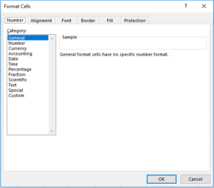
If you find yourself changing the formatting of cells often then using this shortcut could help save some time rather than right clicking format cells. It may not be a huge time saver but if you’re not using the mouse then it’s an easier way to access that menu.

2. CTRL + F1 : Toggle the ribbon

When you’re working with a lot of data often times you’ll need just a bit more space, and hiding the ribbon can help give you see more rows on your page. You can also double-click on the active tab’s name and it will accomplish the same result.

3. CTRL + ~ : Show formulas

If you’re editing a spreadsheet and want to quickly find where there are formulas versus which cells are hard-coded, this is an easy way to show you what is actually entered in the cell, as opposed to what the end value is. The ~ button is normally located next to the 1 on your keyboard.

4. CTRL + ] and CTRL + [  : Showing dependents and precedents

These shortcuts are useful because if you click on a cell that has a formula you can see if there are other cells that are dependent on the cell for inputs somewhere else, or which cells feed into this one. CTRL + [ will show you which cells the active cell depends on, and where its inputs come from, while CTRL + ] will show you if the active cell is used in calculations elsewhere.

You can hit tab to cycle through all the cells that have been highlighted.

It will not show you all the cells if the related cells span multiple tabs, but it can be helpful when looking at formulas and inputs in all other cases.

5. ALT + F1 : Insert a chart

This shortcut can allow you to quickly launch a chart based on the data that you’ve selected. This again may not be a big time saver, but if you’re on a different tab or

Loan and Savings Formulas – PV, FV, and PMT

In a previous post I covered my amortization/depreciation template.

Here I will cover how to do present value and future value calculations that are used in that template. I will start with a savings example. Suppose I want to accumulate $500,000 in savings at the end of 25 years after making monthly payments. I will assume an average interest rate of 3%. My inputs will be as follows:

Present Value (current savings) = 0
Future value (target savings) = $500,000
Number of payments (n) = 300 (25 years * 12 monthly payments a year)
Interest Rate (i) = 0.25% (3%/12 months)

Payment  Calculation


To determine the size of the payment I need to be making to ensure I meet my target calculation, I will need to use the PMT (payment) formula. With the above inputs, my formula will look as follows:

=-PMT(0.0025,300,0,500000)

I enter a negative before the formula to ensure my value will be positive. This yields a result of $1,121.06. I could add an additional argument to say that the payments are at the beginning of the period as opposed to the end. All I need to do is add a another argument with the number 1, as shown below:

=-PMT(0.0025,300,0,500000,1)

The result would be $1,118.26; a difference of less than $3 a payment.

Future Value Calculation


I can test my calculations by now doing a future value calculation. My inputs remain the same, except now I have a payment amount.  The future value formula will look as follows:

=FV(0.0025,300,-1121.06,0)

I have made the payment amount negative so that the formula results in a positive number. My future value equals 500,001.53, confirming that I will reach the target amount with this payment amount. I could also change the payment number from 300 to 150, to determine how much I will have amassed halfway:

=FV(0.0025,150,-1121.06,0)

This tells me I will have a balance of $203,723.81 after 150 payments.

I’ll switch over to another example now. Let’s assume you have a mortgage and want to know what your balance is today. You can use a similar calculation, except this time you will have a negative present value and don’t know your future value (today’s value). Suppose a mortgage of $250,000, a 30 year mortgage with monthly payments (n=360), an interest rate of 5% and payments of $1,342.05 (this can be calculated in much the same way as the payment calculation was done for the first example).

My inputs are as follows (assume I want to know the balance halfway through the mortgage, after payment 180):

Present Value (mortgage amount): $250,000
Number of Payments (n) = 180 (15 years * 12 monthly payments a year)
Interest Rate (i) = 0.4167% (5%/12 months)
Payment = $1,342.05

The formula is as follows:

=FV(0.004167,180,1342.05,-250000)

Again you will notice the present value amount is negative here. This is because this is the amount owing. If this was the same sign as the payment amount the balance would increase rather than decrease. This calculation tells my the mortgage balance after 180 payments, or halfway through the mortgage would be $169,709.77. You may notice slightly different amounts because of the interest rate you use. In the above example I rounded to 0.004167 however if you reference the cell that has the interest rate calculation rather than a hard-coded number you will get a more accurate result.

Present Value Calculation


I will move on now to a present value calculation. In this example, I want to determine what mortgage amount can be afforded based on a specific monthly payment. Suppose I want the monthly payment to be $2,000; the term to again be 30 years; the interest rate to still be 5%. With these inputs I can determine what mortgage amount I can afford based on those assumptions. My formula will be as follows:

=PV(0.004167,360,-2000,0)

In the formula above I again set the payment amount to a negative so that the formula gives me a positive number. The result is a value of $372,563.23.

When doing these calculations you are always better off referencing formulas for interest rate calculation as opposed to hard-coded numbers. As you will notice, even a slight difference in the interest rate can have a big impact on your result, especially when dealing with a large number of payments. I have hard-coded examples in all of the examples here only for illustrative purposes but in practice I would recommend avoiding hard-coding an interest rate.

sum calculation

Using Summation Formulas (SUM, SUMIF(S), SUBTOTAL)

I have saved this sample file here if you would like to look at the data set and have a closer look at how the formulas work.

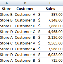
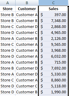
In this post I will cover some simple summation formulas and when best to use them. I have a sample data set that has stores, customers, and total sales.

sum calculation

Summing Total Sales


If I just wanted to total all the sales then the SUM function would accommodate this easily. There is even a summation button on the Excel ribbon to easily do this.

sum ribbon button

It is on the right hand side of the Home tab in the Editing group. It will try to determine which cells you want to sum but you can change this range to what you need.

Since my values are in column C my formula would be as follows:

=SUM(C:C)

Pretty straightforward, all you need is the column that you want to sum (or specific range if you don’t want everything in the column). This returns the grand total of $256,129 from my data set. Another way I could find out the total is if I just highlight the entire column.

sum column

The sum will show in the bottom right corner of my screen in the status bar.

sum status bar

If I right click on any of this area I get the following menu:

customize status bar

If you didn’t see the sum in your status bar this is where you can add it. In my example I could select Minimum and Maximum and then those values would also be calculated for any range that I highlight and show up in the status bar. This makes it easier if you quickly want to see an average, total, min or max by just highlighting a range without having to type a formula each time.

Summing Single Store Sales

But now suppose I just wanted to know the sales of Store A. I could filter the data set, select the column, and see the total in the status bar. But that is a bit tedious to repeat each time if I wanted to see sales by each store. In this case, I could use the SUMIF function.

My formula would look like this:

=SUMIF(A:A,”Store A”,C:C)
      

The first argument, column A, specifies what range I want to look at; the second argument, “Store A”, is what criteria I am looking for; and column C is the final argument, where I want to pull the values from. This formula is saying to look in column A for a value of Store A and add only those related amounts in column C.

Instead of a static reference for Store A I could reference a cell instead, and that would make it easier to apply this formula to multiple stores without having to change the name manually each time.

In the above example assume my store name is in cell E6. If I have the store names going from cell E6:I6 then I could use the following formula:

 =SUMIF($A:$A,E6,$C:$C)

You will notice I have frozen some of the cells as well. This will allow me to move my formula across without the ranges changing. Below are what my results look like:

sumif calculation function

Summing Sales by Customer and Store

Now, consider a scenario where I wanted to do a summary of sales by stores and customers. Here I can use the SUMIFS function (only available to Excel 2007 and newer versions). In the formula below I have stores in cells G12:J12 and customers in cells F13:F16:

 =SUMIFS($C:$C,$A:$A,E$12,$B:$B,$F13)

I can copy this formula and it will be updated based on what store and customer intersect at that point. The summary will look as below:

sumifs formula calculation

Unlike with the SUMIF function, the first argument here is the range I want to sum, which is column C. The next argument is the range for my first criteria to look up, column A, followed by the criteria I want to match, which in the first formula is cell E12 (Store A). The next two arguments relate to the next criteria range which is column B for the customers and the customer to be matched which in the formula is cell F13 (Customer A).

With the SUMIFS function you can add more criteria than just two. Simply just add another comma and in the next argument specify the range, followed by the criteria. You can keep adding to it as you need.

How the SUBTOTAL Function Works

Unlike the SUM function, the SUBTOTAL function will perform a calculation based on the filters you have applied (if you have none, it will perform a calculation on all the data in the range). The SUBTOTAL function also has an added argument to tell it what type of calculation it should do:

subtotal functions

In the below formula, I am going to total column C again, as I did in the SUM formula initially. However, the additional argument I need in the SUBTOTAL function is defining the calculation. Since I am going to just do a sum, I will set the argument to 9. My formula looks as below:

 =SUBTOTAL(9,C:C)

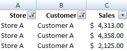
Now, if I were to use filters to show only Store A and Customer A, the SUBTOTAL formula would return the same result as the SUMIFS function did for the intersection of Store A and Customer A.

subtotal filters

My formula returns a value of $10,796 with the above filters, which matches the result from the SUMIFS formula. The SUBTOTAL function is useful when you are always using filters since it will take those filters into account as opposed to the SUM function which will ignore them. If you don’t use filters then it won’t make a difference.

How to Freeze Panes

Freezing panes in Excel is useful when you want to still see certain rows or columns as you scroll through a large data set. Without doing so you could easily get lost in your data trying to figure out which header or category the value you are looking at belongs to.

Under the View tab select Freeze Panes and if panes are frozen you will see an option to unfreeze panes. Otherwise you can choose to select to freeze panes, freeze top row, or freeze first column. Freeze top row will ensure that row 1 is frozen is you scroll down and ensure you will see your headers. Freezing the first column will make sure column A is always visible as you scroll to the right.

Now but what if you wanted to freeze both rows and columns, or multiple rows or multiple columns? That is where you would just use the regular Freeze Panes option. The key here is to select the correct point of intersection. When you press freeze panes the active cell will determine which rows and columns are frozen. Any rows above and columns to the left of the active cell will be frozen.

For example, if you wanted to freeze just the first row, you would select cell A2. Since there is nothing to the left of it, it would only freeze row 1 which is above.

Above I have highlighted the frozen row as well as which cell I would need to select to achieve that.

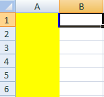
If you wanted to freeze just column A, you would select cell B1. Since nothing is above row 1, only column A is to the left of B, so only A would be frozen.

See above for the highlighted column and what cell I would need to select to freeze it.

 If you wanted to freeze column A and row 1 then you would need to select cell B2 since row 1 is above that cell and column A is to the left. See below:

Similarly, if you wanted to freeze the first two columns and the first two rows you would select cell C3 – see below for results

Simple VBA Tricks

A couple quick snippets of VBA code that can help you impress your friends although might not have much real utility.

First up: have Excel speak to you

Application.speech.speak “text”

Where text is what you want Excel to say. Just like with any other code you can of course use variables for this to alternate. You could create a list to cycle through various messages as well.

Another one: opening a URL

ThisWorkbook.FollowHyperlink “http://www.google.com”

The above code will open Google when triggered in the default browser.

Highlight Alternating Rows or Columns

This post will show you how to create the effect of highlighting alternating rows, which sometimes makes it easier to read a data set.

In order to accomplish this, first select all the cells in the worksheet and then select New Rule under conditional formatting.

For the new rule you will need to select the last option to use a formula. The formula we will need to use is as follows:
=MOD(ROW(A1),2)=1
The MOD function calculates the remainder after division and has two arguments, the number to be divided into, and by what number. 
Using ROW(A1) means the reference will change depending on the location of the cell, meaning it will encompass every row in the selection. Using 2 as the divisor will help identify if the row is as odd number or even. If you’d rather highlight columns than rows, use the COLUMN function.
The formula will be true if the remainder is 1, meaning the row is an odd number (e.g. highlighting will start on the first row). If you want highlighting to start from row 2, just change the 1 to a 0, since even rows will have no remainder.
Once the formula is set, click on Format to determine the appearance of the alternating rows.
I select a light blue colour for the alternating rows
After I press OK this is the result of my conditional formatting:
If you don’t want to apply the formatting to all the cells or want to change the range, under conditional formatting select manage rules
There you will see a field where the formatting Applies to. Here you can change the range you want the formatting to apply to.