4 Biggest Annoyances of Pivot Tables and How to Fix Them

Pivot Tables are great tools, especially for quickly summarizing data and allowing you to avoid entering in complex formulas to do so. However, they aren’t perfect and definitely have their quirks about them.

Here are four things that most users aren’t crazy about, and how to fix them.

The layout

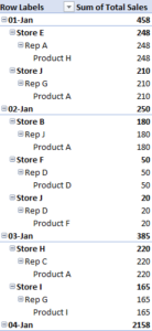
When you create a pivot table it puts the table into a layout that is less than optional for spreadsheets. It’s not only hard to use for any other purpose, but it’s also not the easiest format to read. I always prefer a format that resembles more of a spreadsheet itself, in a grid format, without the indented rows.

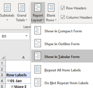
To change the format, go to the Design section of the PivotTable Tools and select Report Layout and select Show in Tabular Form

This is what the pivot table looks like after the change:

This might still look a little cluttered, but what you can also do is get rid of any subtotals by simply right-clicking on the Total and unchecking the Subtotal button, and then it’s a bit cleaner:

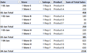
The table still needs a little work for me, and that brings me to the second issue:

Labels do not repeat

You’ll notice that the value in the date field only shows up once. And so if I had many entries for a given date there would be a lot of blank values in the first column. Again, this is not ideal for a large data set and so this is where I’d like to make a change as well.

I go back to the Report Layout section, except this time I select the option to Repeat All Item Labels

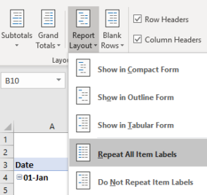
Now my table looks like this:

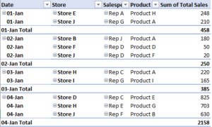
This is what I would hope the pivot table looks like right off the bat. Unfortunately, Microsoft does not agree and opts for the indented version with subtotal at every section and no repeating values.

But that’s not all, there’s another little nuance you may notice when it comes to pivot tables:

Formatting won’t stay consistent

You’ll notice that in the sales data, I have a total of 2158 for January 4th. Anytime you’re dealing with numbers in the thousands, you’ll probably want some formatting that shows a comma in there just to make the numbers more readable. However, if you simply select the entire column and change the formatting, it will revert back to the default if you refresh the pivot table after adding more data.

What you need to do is actually change the field settings. To do this, right click on any of the numbers in that column and select Value Field Settings.

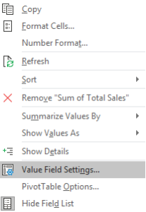
From there, select Number Format and then select the format you want it to show up as. Doing this will ensure the formatting won’t change when you refresh the data.

Tip: if you routinely make these changes like I do, you may want to check out the add-in I created which will make all these changes for you at the click of a button.

This brings me to the fourth most irritating item when it comes to pivot tables:

GETPIVOTDATA

By default, when you reference a number in a pivot table, it will auto-generate a formula called GETPIVOTDATA. In most cases, you probably won’t find this helpful, especially if you just want to reference some pivot table values elsewhere in your workbook. If you just want to reference cell E4 and copy the formula down, you’ll need to adjust the pivot table settings, as the GETPIVOTDATA will make it a bit painful to accomplish this.

Back under the PivotTable Tools section, select the Analyze tab and on the Options menu on the left-hand side, uncheck where it says Generate GetPivotData

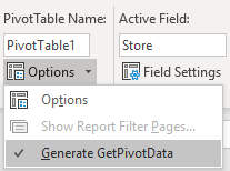
Now you can reference values from a pivot table the way you would any other cell in your workbook.

If you have any other frustrations with pivot tables, please share them in the comments.