How to Use GetPivotData

For many users, the GETPIVOTDATA function in Excel is a nuisance and people are often looking for how to turn it off, rather than to actually use it. It can be a bit of a clunky formula, to say the least, but it can be very useful once you’ve learned how to use it effectively, which is what I’ll show you to do in this post.

Using GETPIVOTDATA to extract data using a single criterion

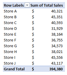
I’ll start with a simple pivot table that just shows stores and sales:

If I select the cell that has the sales for Store A, Excel populates the following formula:

=GETPIVOTDATA(“Total Sales”,$B$4,”Store”,”Store A”)

Let’s break down the different parts of this formula:

“Total Sales” is the first argument, and it is the name of the data field that I’m pulling my numbers from.

$B$4 is where my pivot table is located. However, this specific cell doesn’t matter, as long as the range is somewhere on your pivot table. For example, I could use B5 or B6; as long as the cell is located on the pivot table, the result will remain the same. The cell also doesn’t have to be frozen. However, if the range refers to a cell that isn’t on the pivot table, you’ll get a #REF error.

“Store” is the third argument, and it’s the field that relates where the “Store A” item is found, which is the last argument of the formula.

In essence, the GETPIVOTDATA starts with selecting the field you want to pull data from, the second argument pointing to somewhere on the pivot table, and with the third and fourth arguments relating to the relevant criteria. Think of it similarly to how you might use a SUMIFS function where you first specify what you want to sum, and where you can keep adding criteria to it.

If I only used the first two arguments of the GETPIVOTDATA function, it would return the total for the entire pivot table:

=GETPIVOTDATA(“Total Sales”,$B$4).

This would give me a value of 394,380 – which is the total of everything in the pivot table.

Using multiple criteria in the GETPIVOTDATA function

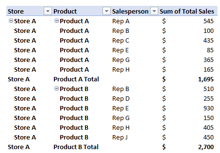
Let’s make this calculation a bit more complex and add both a product field and one for the sales rep as well:

If we want to pull the sales that Rep A had for Product A in Store A, that means we now have three criteria instead of just one. The good news is that all we have to build off the previous formula:

=GETPIVOTDATA(“Total Sales”,$B$4,”Store”,”Store A”)

To follow the pattern, what we’ll want to do is add the field name followed by the item in the field that’s our criteria. That means we need to add the “Product” field followed by “Product A” for the item:

=GETPIVOTDATA(“Total Sales”,$B$4,”Store”,”Store A”,”Product”,”Product A”)

Now, if we want to make it more complex and add Rep A as another filter, then it’s just a matter of adding the “Salesperson” field and “Rep A”:

=GETPIVOTDATA(“Total Sales”,$B$4,”Store”,”Store A”,”Product”,”Product A”, “Salesperson”,”Rep A”)

As you can see, you can add in as many criteria as you like. The key is just making sure that the field names you use match exactly what the fields are called on your pivot table. Otherwise, if the field cannot be found or if it is misspelled, you’ll get a #REF error.

Making the GETPIVOTDATA dynamic

Entering in all these fields is not optimal, and the real value in using GETPIVOTDATA is by being able to make the results dynamic and using variables to do the work for us.

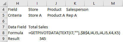
To do this, I’ll set aside cells for both the field names as well as the criteria. Here’s how the new, dynamic formula would look now:

What you’ll notice is the GETPIVOTDATA now has nothing hardcoded that you’d have to change in the formula. Instead, you could change the fields in rows 4 and 5 instead. Let’s breakdown the formula in a bit more detail to see how it works:

=GETPIVOTDATA(TEXT(I7,””),$B$4,I4,I5,J4,J5,K4,K5)

The first argument, TEXT(I7,””), references the Total Sales field in cell I7. The reason I use the TEXT function here is that the value needs to be forced into a text format, and by using “” as the second argument in that function, it will keep everything the same.

The following argument, $B$4 still just has to point to somewhere on the pivot table. Unless you move your pivot table, you won’t need to change this argument.

The following arguments: I4,I5,J4,J5,K4,K5 all relate to the cells that have the field and criteria data. Change the values in those cells and the formula will automatically update, rather than having to fumble around and make changes in the actual formula.

Limitations

There are some important limitations that you should be aware of when using GETPIVOTDATA.

Blank values will cause errors

If in the example above you want to use fewer than three criteria, you’ll have to modify the formula, otherwise, you’ll get a #REF error if you simply clear the variables and make them blank.

Data must be visible

Another important thing to remember: if your pivot field isn’t showing the data, the GETPIVOTDATA won’t be able to use it.

Since I’ve removed the Salesperson field from the pivot table, I can no longer use that as part of the criteria in my GETPIVOTDATA formula, and hence is why there is now a #REF error in my result. Even though it is still in the dataset, GETPIVOTDATA will only be able to extract from information that is visible on your pivot table.

Order is important

The order that the fields show on the pivot table will impact how you can use GETPIVOTDATA. For example, if I have Store, then Product and then Salesperson in my pivot table, I have to take that into account when creating the GETPIVOTDATA formula; I can’t just use GETPIVOTDATA to use criteria from the Store and Salesperson fields and skip over Product. I can, however, pull the totals for Store and Product and then just not include Salesperson, since I’m not following a different hierarchy than what’s shown in the pivot table.

Too many fields will make it difficult to summarize totals at lower levels

The GETPIVOTDATA function can be very particular, especially when it comes to hierarchy. For instance, you won’t be able to total sales by rep for everything in the pivot table if you’ve got the store and product fields shown higher up in the hierarchy; you’ll need to incorporate those fields into your calculation. That means adding all those combinations where the sales rep is found, which isn’t optimal. I can’t just say I want to see the total sales this rep made, forget all the product and store combinations that come above it in the hierarchy. The easiest way would be to simplify the pivot table to remove those fields or make the Salesperson field at the top of the hierarchy, and then it would be possible to do that by just using one criterion.

Why formulas may be a better option

GETPIVOTDATA has its strengths, but as you can see, it also has many weaknesses and limitations. This is where using formulas like SUMIFS can be a lot more useful if you’re comfortable using them. GETPIVOTDATA can be useful for pivot tables that aren’t going to move or change and it could also be a bit quicker than a lookup or other function. If you’ve got a lot of cells that you need to populate, SUMIFS may just end up slowing down your spreadsheet too much, and you may find it easier just having multiple pivot tables with different views instead.

At the end of the day, if you hate GETPIVOTDATA and prefer a simpler approach like just using lookup functions to get your data, this post will show you a simple way to get rid of it when selecting cells on a pivot table.

If you liked this post on How to Use GetPivotData, please give this site a like on Facebook and also be sure to check out some of the many templates that we have available for download. You can also follow us on Twitter and YouTube.