H2Eerror1

Deleting a Formula in Excel? Do This First

When you’re dealing with complex spreadsheets in Excel, it can sometimes be difficult to tell which cells are safe to delete and which ones you need to keep to ensure everything is working properly. Even cells that look empty could contain formulas. And deleting them can cause problems and wreak your spreadsheet. Before you delete a formula, there’s one thing you can do to prevent that mistake:

Check for dependent cells

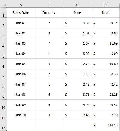
If you’re not sure if a cell is okay to delete and if it has any other cells that depend on it, you can check for dependents. Before deleting a cell, you can click on CTRL + ] which will highlight any cells that use the active cell in a formula (on the current sheet). Here’s a sample spreadsheet that lists price, quantity, and multiples them to get to a total price:

Spreadsheet that calculates the total by multiplying price by quantity.

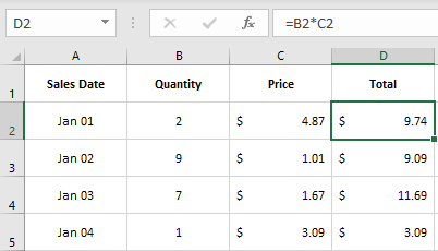
The formula in column D multiples the value in B by C. So that means the value in D depends on the values in C and B (the exception is the subtotal, which depends on the values above it). If I select cell C2 and click on CTRL+], it takes me to cell D2:

The dependent cell is highlighted.

If there is more than one cell that depends on the active cell, then Excel will highlight all of them.

What if there aren’t any dependent cells? In that case, you’ll get the following message:

Message box saying no cells were found.

If you get this message, that means you’re safe to delete the current cell as nothing in the current sheet links to it. However, the one limitation of using the shortcut is that it may not be easy to see all the cells that depend on that one cell. It also won’t tell you if there is a cell on another sheet that uses it.

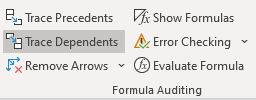
What you can do is use the Trace Dependents button in Excel, which is on the Formulas tab:

Trace Dependents button.

By clicking on this button, arrows will now show up telling me exactly where the dependent cells are:

Arrow showing the dependent cell.

In this situation, the arrow clearly shows an arrow pointing to cell D2. Let’s say I also use the cell in a formula in some place far off in a the same sheet:

Arrows showing multiple dependent cells.

Another line will point to the other cell. If you have a large data model that goes on for many rows and columns, it may not be obvious where the dependent cells are if you use the shortcut key. Using the shortcut can be helpful as a quick check but if you actually want to see all the cells that use the active cell, you’re better off clicking the Trace Dependents button.

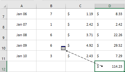
Next, let’s go to the subtotal. Here, let’s assume I’m using this total somewhere on another sheet. Using CTRL+] won’t help me much in this case as it will tell me no cells were found (assuming no cells on the current sheet link to it). But if I click on Trace Dependents, it will show that there is a dependent cell on another sheet:

Dependent cell is on another sheet.

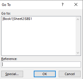
If you double-click on the dotted line (the portion that’s within the cell), the following box will pop up:

Go to box showing where the dependent cell is located.

This tells us that there is a dependent cell on Sheet2, cell B1. I can go there manually or I can click on the selection and then press OK. Then it will take me directly to the cell:

Dependent cell that links to another sheet.

This isn’t practical on a wide scale as you would have to go one by one and you could have arrows going all over the place. But if you’re not sure about a certain cell, using the Trace Dependents button can be a quick way to see if it’s safe to delete the cell.


If you liked this post on 1 mistake to avoid when deleting formulas in Excel please give this site a like on Facebook and also be sure to check out some of the many templates that we have available for download. You can also follow us on Twitter and YouTube.

H2Epercentages

How to Calculate Percentages in Excel

When doing any kind of data analysis, it’s important to be able to pull in not just raw data but also to show percentages. From a period-over-period percent change to how much an item represents of a total, showing a percentage can give readers multiple different viewpoints. Below, I’ll show you how to calculate percentages in Excel and to give your data more context.

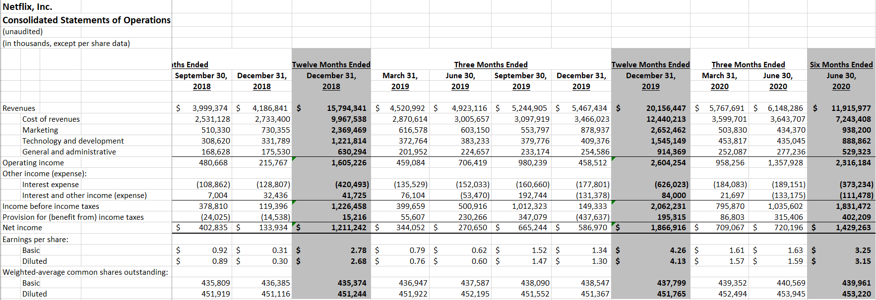
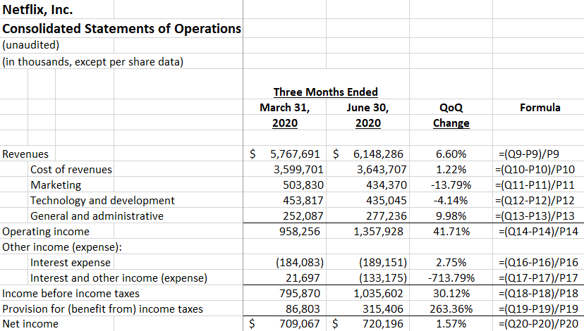
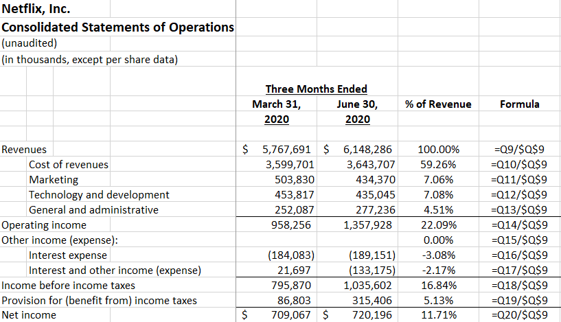
In this example, I’m going to use data from Netflix’s most recent quarterly results. The streaming giant always releases its numbers in a friendly Excel format, making it easy to analyze the data. Here’s what its income statement tab looks like, unchanged for the second quarter of fiscal 2020, which includes previous periods:

Netflix income statement in Excel.

Showing period-over-period changes

Netflix’s numbers look impressive — $6.1 billion in revenue for the quarter ending June 30, 2020. However, that number on its own may not be very helpful. One way to add some context is to calculate the percentage change to show the increase or decrease from a previous period, aka its rate of growth.

I’ll add a column next to those quarterly results and add a formula that shows the percentage difference from the previous quarter (ending March 31, 2020). To calculate the percent change, all I need is to take the difference and divide it by the old number, or base amount. A good way to remember this is: (new-old)/old.

In this example, column Q contains the quarterly results for June 30 and column P is the previous period. And the revenue is in row nine. The formula for the first item looks as follows:

=(Q9-P9)/P9

Where Q9 is the new total, while P9 is the old number. This gives me the following:

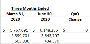
Quarter over quarter change.

The $0 isn’t really helpful here, and it’s also not a dollar amount. Excel’s just defaulted it to that format based on the other numbers. To properly show it as a percent change, I need to change it to a % format. It’s as simple as selecting the entire column and clicking on the % sign on the Number tab:

Number group in Excel.

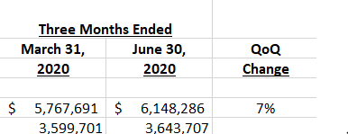
That will now give me the following results, after centering the column:

Quarter over quarter change in percent format.

However, this still may not be ideal. If I want a bit more detail, such as to show multiple decimal places, you’ll again want to go back to the format section and select the item to add decimal places:

Add decimal places button.

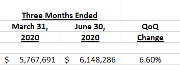
Clicking on this button twice will now give me a couple more decimal places:

Percent change with two decimal places.

Now, with my percentage change looking correct, I can copy the formula down for the rest of the items:

Quarter over quarter percent change across all items.

Showing the percentage of a base amount, or grand total

Another way you may want to show a percentage is how much an item makes up of a total. One common way to analyze financial statement is to look at items as a percentage of revenue. A company’s profit margin, for instance, takes its total profit and divides it by revenue to determine what percentage of its top line makes it through to the bottom line.

How to calculate percentages in Excel when just looking at how much an item makes up of a grand total is an easier process. In this example, the calculation just takes the current item and divides it by revenue. The key is just freezing the denominator, which in this case is revenue. Here’s how the formula looks like:

Percent of revenue by line item.

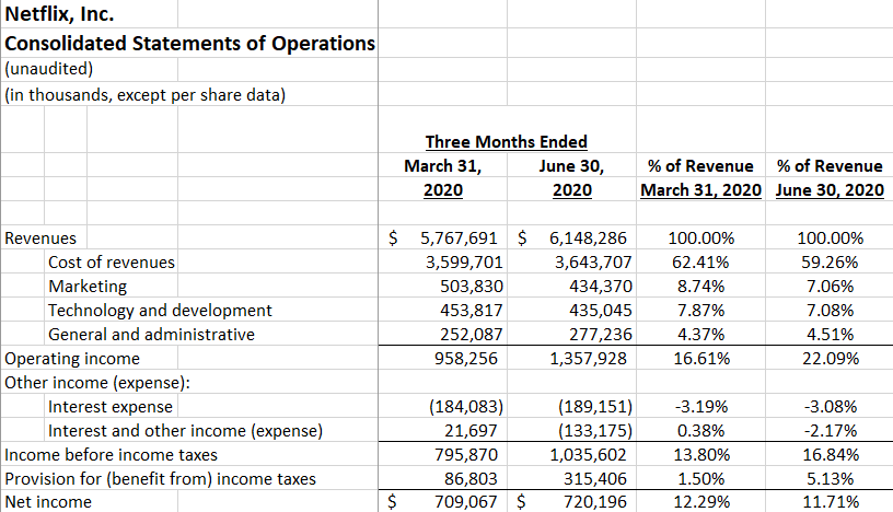
Using the % of revenue analysis, it’s easy to see that operating income was 22% of revenue and Netflix’s profit margin was 11.7%. Replicating these formulas for other periods can help compare multiple periods to see the % of revenue trends. Here’s how the current quarter looks against the previous one when looking at the percent of revenue:

Multiple periods percent of revenue analysis.

Compared to the earlier quarter, Q1, the profit margin becomes a bit less impressive in Q2 as it’s declined from the previous period. Despite a stronger overall Q2 performance, a higher tax bill led to a smaller overall profit margin than in Q1.

As you can see, by adding percentages to your analysis you can create very different viewpoints and add a lot more context to the numbers.


If you liked this post on how to calculate percentages in Excel, please give this site a like on Facebook and also be sure to check out some of the many templates that we have available for download. You can also follow us on Twitter and YouTube.

vlookup1

3 Reasons You Should Still Use VLOOKUP

Many people will tell you that you should use INDEX/MATCH instead of VLOOKUP or that you should use a new function like XLOOKUP instead. But you shouldn’t be so quick to ditch arguably the most popular function on Excel as it’s still very useful. Below are just three reasons why VLOOKUP is still incredibly valuable:

1. It’s really quick to set up

If you’re using a combination of INDEX/MATCH, you’re going to have to use two functions, correctly set them up and nest one inside the other. Especially if you’re not used to it, it can take some time to set it up. Sure, it’s not like it’s going to take hours or even minutes to do, but if you need a quick lookup and VLOOKUP can do the job, why not just use it? Here’s how quickly it takes to set it up:

In the above example, I do a VLOOKUP in about five seconds. If you’re setting up INDEX/MATCH, you might still be trying to figure out which column to use for your MATCH argument. Being able to do VLOOKUP without almost thinking is what makes it such a great function, its speed is through the roof. Since you know the first column of your range is where you’re looking up values, it simplifies the process of selecting the columns and then you’re just counting how many columns over you’re extracting data from.

A couple of ways I expedited the formula above is by not typing out the entire function name (just entering VL and then tab to autocomplete the name), using 0/1 instead of typing out True/False and by not closing the last “)” as Excel will automatically do this for you.

Sure, it won’t work in all scenarios such as if you need to go left, that’s a well-known limitation of VLOOKUP. But as long as that’s not the case, there’s really no reason you need to bother with INDEX/MATCH when VLOOKUP will do the job. I’ve been using Excel for decades and I still love to use it when I can because it’s so easy to set up.

2. VLOOKUP is very versatile and will work on old versions of Excel

VLOOKUP may not be able to go left, but it can do wildcard searches and it can work if you need to pull the closest value — this is really useful if you’re dealing with tax brackets or anywhere that you’re looking for the closest value without going over (e.g. where you set the last argument to TRUE to look for approximate matches). While many people may use it strictly for exact matches, VLOOKUP is much more powerful.

And here again, using VLOOKUP in these situations is likely going to be no more difficult than the alternatives. While the temptation may be to use an exciting new function like XLOOKUP, the one big disadvantage is that it’s not available on older versions of Excel. With VLOOKUP, even if you’re working on a version that’s 20 years old you won’t have to worry about whether the formula will work.

3. Ease of use makes it ideal for training novice users and making templates with

Not only is VLOOKUP easy to set up, but it’s easy to understand compared to other, more complicated functions. If you’re making a template or need to train users, you don’t want to worry about them knowing complex formulas, especially when it involves nesting functions. Or telling them about a formula that may not work on their version of Excel. VLOOKUP’s also a good stepping stone for beginners to get them accustomed to how Excel formulas work.

Complex formulas are easy to break and harder for inexperienced users to fix. That’s why VLOOKUP’s ease of use is a key reason it’s worth using. If you’ve ever had to fix someone else’s formulas, you can definitely appreciate that keeping formulas as simple as they need to be can go a long way in making it easy to maintain and fix a spreadsheet.


If you liked this post on why you should still use VLOOKUP, please give this site a like on Facebook and also be sure to check out some of the many templates that we have available for download. You can also follow us on Twitter and YouTube.
5ways

5 Ways to Count and Extract Unique Values in Excel

There are many ways you can pull and count unique values in Excel, and below, I’ll show you five ways you can do so and when you should use each method.

For this example, I’m going to use a dataset from data.gov relating to consumer complaints about financial products. It’s a large list and by listing the unique values we can see how many different complaints there are and which are the most common ones.

Using the UNIQUE function to extract values

The UNIQUE function isn’t available on all versions of Excel. You can try to type it in as a formula to see if you have access to it. If you’re able to use it then that’s great news, because this is the easiest way to pull unique values.

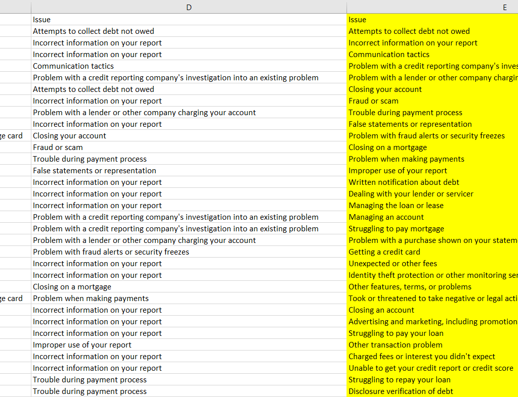
In my data set, I want to extract all the unique issues customers have had. I can quickly generate a unique list of values by using this function and just selecting the entire range of cells in column D. The formula is as simple as this:

=UNIQUE(D:D)

It returns an array and the unique results are now in the column where I entered the formula (E) and I’ve highlighted the list in yellow:

unique values using the unique function.

This gives me the entire list of unique values but it doesn’t tell me how many unique items there are. I could, of course, just use a count function to tally up all the values in column E. But there’s also another, more efficient way to do that. I can enclose the UNIQUE function within the COUNTA function that counts nonblank cells. Here’s what that formula looks like:

=COUNTA(UNIQUE(D:D))

This formula tells me that there are 167 unique values in column D. I don’t even need to first run the UNIQUE function on its own, I can do this all in one cell and quickly get the number of unique values in the list. This is by far the simplest and most elegant way to do this in Excel.

If I wanted to see the number of times a unique value appeared on the list in column D, I could use the following formula:

=COUNTIF(D:D, E2)

Where E2 is the issue that I want to count.

Let’s move on to another approach, one that’s more common in newer Excel versions.

Using the remove duplicates button

Another way that you can pull the unique values from a list is by clicking on the Remove Duplicates button located on the Data tab:

remove duplicates button

However, the caveat here is that this button will actually remove items from the existing list that aren’t unique. And so what you’ll want to do first is copy your list of values to another column, and then select that column and click on the button.

At that point, you’re back to having to count the number of duplicates in the list. A function like COUNTA could do the job. And then to tally the totals by item would involve using the COUNTIF function again.

Going old school with the advanced filter trick

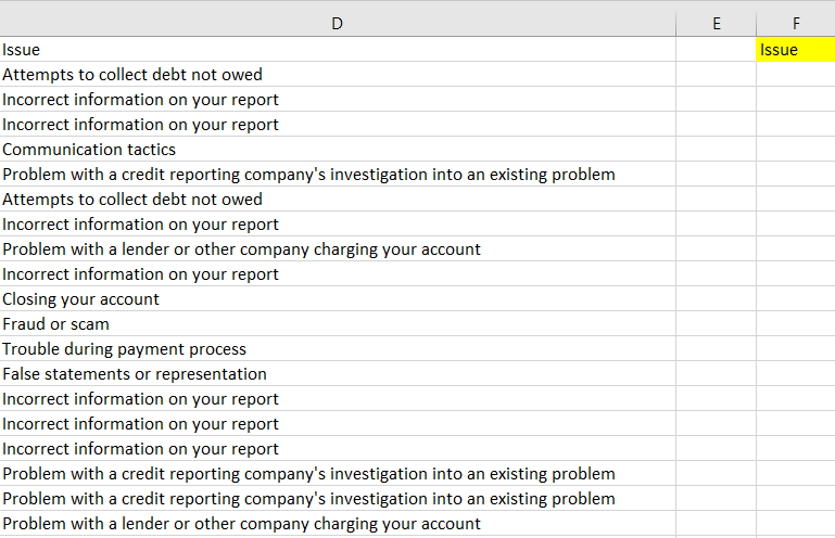
If you’ve worked on older versions of excel where you didn’t have the luxury of buttons filtering out duplicate values for you, you may have used an advanced filter. How this works is you enter the header into some other adjacent range like so:

Using the advanced filter to create a unique list of items.

Then, click on a value in column D, and then click on the Advanced Filter button on the Data tab, which looks like this:

Advanced filter button

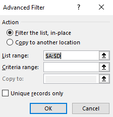
The advanced filter should automatically detect the range you’re looking to filter. You’ll then see a pop-up box as follows:

Advanced filter pop-up box.

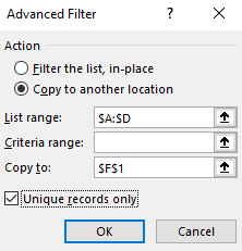
I’ll tick off the Copy to another location button and I’ll select F1 which is where my header in the adjacent range is located.

Filling out the advanced filter pop-up box.

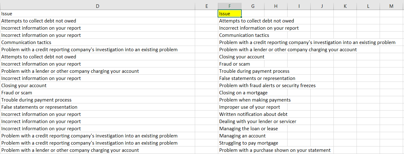
Ticking off the box for Unique records only is what makes the filter pick up only the unique values, which after clicking on OK will now populate column F:

A list of unique values after running the advanced filter.

The advantage of doing it this way is you don’t have to copy a list and then remove duplicates, and essentially the end result is the same. This is the method you may want to use on older versions where you don’t have access to the newer options.

There’s also one another way that you can filter out unique values, and it’s one of the more common approaches I’ve seen.

Using pivot tables

I cringe a little when I see people using pivot tables solely for the purpose of create unique lists. It’s overkill, especially given the methods listed above that do the job just fine. But it does do the job and if you’re wanting to do some sort of analysis, it’s a great way to do it all in one shot.

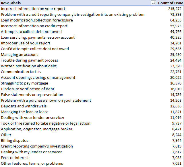
For example, using my data set I can quickly turn it into a pivot table and not only create a unique list but also do a count by issue and sort it from highest to lowest:

Creating a pivot table.

Rather than using COUNTIF, I can just let the pivot table do the counting for me. If you want to calculate the number of unique values, you can again use the COUNTA function. You can use it to count the number of values in the Row Labels section of the pivot table. You’ll of course want to adjust for any headers and grand totals to ensure you aren’t counting too many rows.

Use our FREE Add-in!

Whether you need to count unique values or create a list of them, you can easily do them through our free add-in. You don’t have to worry if you have the right version of Excel and it’ll work with the click of a button:

Howtoexcel.net free add-in that can filter and count unique values.

And that’s just one part of a much larger set of macros and buttons that can simplify your workflow:

Complete list of macros on the howtoexcel.net add-in.

When should you use a particular method?

There are many options to choose from here when generating a unique list of values. Here’s a quick breakdown of each method and when you’ll want to use each one:

  1. The HowtoExcel.net Free Add-in. This will simplify many of your tasks beyond just populating and counting unique values.
  2. The UNIQUE function. Outside of the add-in, this should be your go-to option if it’s available on your version of Excel. It’s easy and quick to not only generate a list of unique values but to also count them. The advantage of this method is that it will also auto-refresh if your data changes since it’s a formula. You won’t have to re-run the formula to get a fresh list of unique values.
  3. The Remove Duplicates button. This is the next-best option to use if you aren’t able to use the UNIQUE function. It involves just the click of a button and you just need to remember to copy the list.
  4. The Advanced Filter. Use this if you’re working on an old version of Excel and don’t want to install an add-in.
  5. A Pivot Table. There’s no reason to use this method unless your list of values changes often and you need a quick way to refresh the list. However, if you’re also looking to analyze the data then using a pivot table could quickly jump to the top of this list as it’ll help you sort by unique values and also do calculations very quickly.

If you liked this post on how to extract and count unique values in Excel, please give this site a like on Facebook and also be sure to check out some of the many templates that we have available for download. You can also follow us on Twitter and YouTube.
auotfilldata

How to Autofill in Excel

There are many ways you can speed up data entry in Excel. Using autofill can be particularly helpful because Excel can normally figure out patterns and the formulas that you’re going to want to enter. It can save you lots of time from having to manually enter values or formulas yourself. Below, I’ll show you how you can autofill values and formulas in various situations and how you can also use flash fill.

How to use autofill

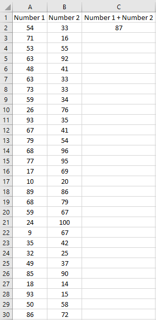
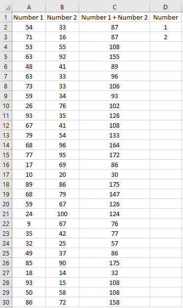
Automatically filling in data is easy in Excel and it’s as easy as double-clicking. Let’s start with a very basic example. Here’s some data I’ve entered using a random number generator:

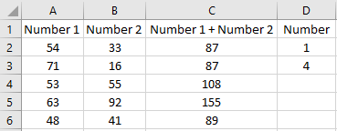
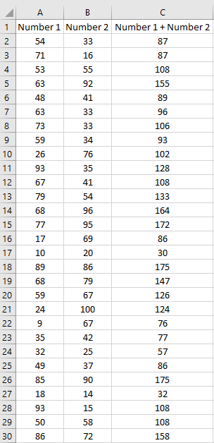
Data entered in Excel before running autofill.

The formula in column C is just adding the corresponding values in columns A an B. It’s a simple formula but that doesn’t mean I want to enter it in repeatedly. To save me the the hassle having to do that, I’ve got a couple options.

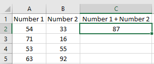
The first is to double-click on the edge of the cell that has the formula in C2:

Selecting a cell in a data set.

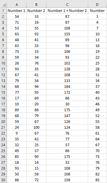
You’ll notice on the bottom right corner there’s a square there. If you hover your mouse over it your pointer will turn into a black cross. When that happens, double-click and excel will autofill the same formula all the way down to the rest of the rows that you’ve filled in:

Data after the autofill has been run.

You could also manually drag the corner down rather than double-clicking it.

Alternatively, if you want to specify how far down you want to autofill then there’s another approach you can take. Start by selecting your formula as well as how far down you want to copy it:

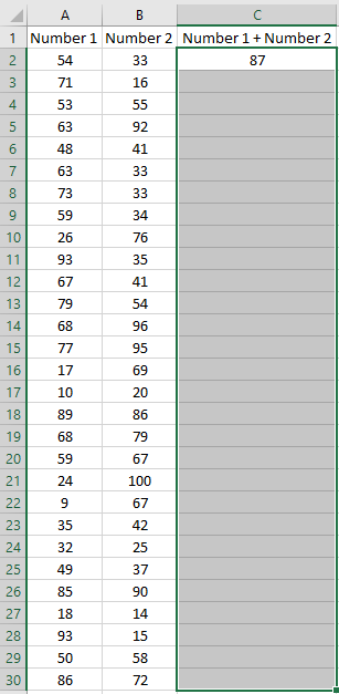
Selecting the cells you want to apply the autofill to.

On the Home tab, in the Editing section, there’s a Fill button I can click on which will give me some options:

Fill button options in Excel.

Clicking on the Down button will autofill the cells I’ve selected with the formula that I entered in the first row. The result is the same as when I double-clicked in the corner of the cell.

The main advantage of doing it this way is if you don’t want the formulas to copy all the way down to where your data ends. It’s not a situation I’ve ever come across and double-clicking is a lot more intuitive and a much simpler approach.

Filling in values

It’s not just formulas that Excel can autofill, it can even work on values. I’m going to add some numbers to my data set:

Numbers added to the data set.

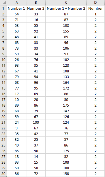
If I try and autofill by double-clicking on the corner of cell D3 this is what happens:

Autofill working incorrectly.

Excel didn’t figure out that I wanted to keep on incrementing by 1 and instead it just copied the number 2 all the way down. When it comes to autofill, you can help Excel by selecting more data:

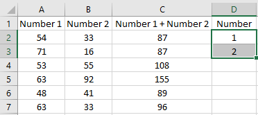
Selecting multiple cells before running the autofill.

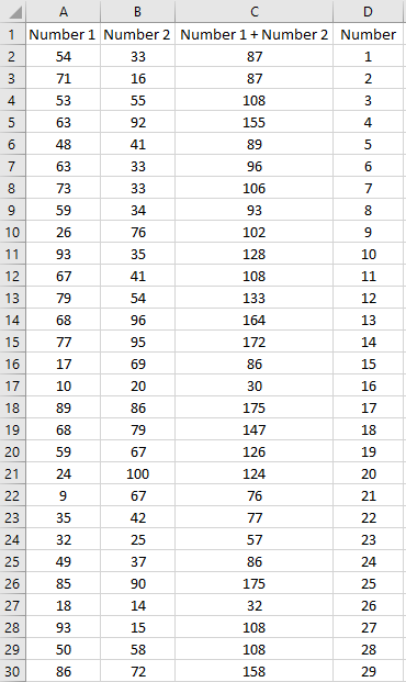
I’ve selected the first two values in the data I want to autofill. Now, when I double-click and autofill from D3, here’s what happens:

Autofill working correctly after multiple cells selected.

Now that I’ve given Excel more of a pattern to work with, it’s figured out what I wanted to do. Even if I select an odd pattern like this:

Autofilling an unusual pattern.

Excel is still able to complete the pattern:

Autofilling by incrementing by three.

Autofill works also works with dates

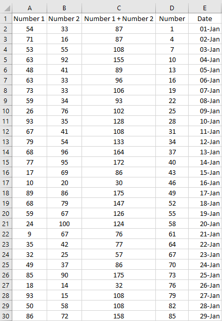
Just like with numbers, Excel can figure out the pattern if I’m working with dates. Here’s a scenario where I’ve only got one date entered in: January 1

Autofilling dates.

If I autofill the rest of the data, it’ll increment by one day:

Autofill increments by one day at a time, by default.

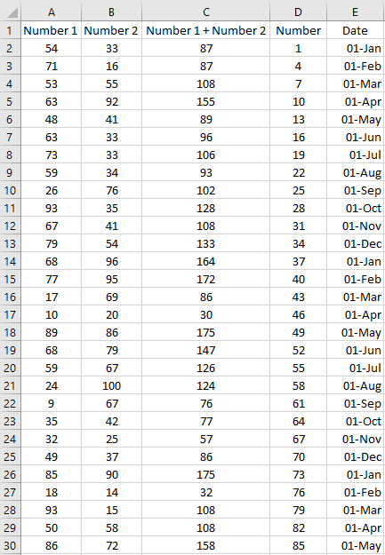
If I don’t want to increment by one day, I can increment by month by giving Excel more data to generate a pattern from:

Multiple dates entered in Excel for autofilling purposes.

Now, using that selection, Excel knows to auto fill the remaining data by one month intervals:

Autofill incrementing by one month at a time.

Flash fill can even figure out your patterns without formulas

Now, let’s switch over to using flash fill, which can almost read your mind. In the following scenario, I have not entered any formulas in the data below:

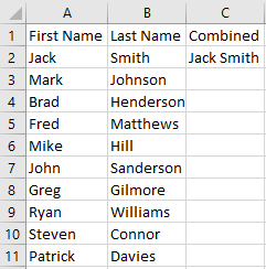
Combining names in Excel.

The value in column C is supposed to be a combination of columns A and B joined together by a space. Without a formula, simply using autofill and double-clicking isn’t going to help in this situation, it’ll just copy the value in cell C2. This is where using flash fill can take you to the next level. If I select the value in cell C2, I can go back to the Fill button and this time select Flash Fill:

Selecting flash fill from the fill menu.

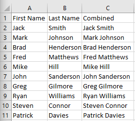
And here’s the result:

Data after running flash fill.

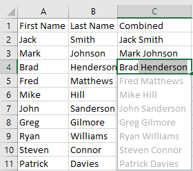
Incredibly, Excel’s filled in the remaining data and pattern with only one cell to work with and no formula entered. Even if I start entering the data manually, Excel will ofter to help me, showing me that it can fill in the pattern for me:

Excel offering to fill in the remaining values.

If I want to accept Excel’s help, I can just click on Enter and it will fill in the remaining cells. Excel doesn’t always get it right, but when it does, it can be a significant time-saver, especially if you’ve got lots of data to enter.

Why you may not want to use flash fill

Although flash fill can save you some time like in the example above, it won’t always work how you may hope. And relying too much on it can prevent you from learning how to use concatenate or other formulas that can make you more efficient in the first place.

It’s always better to use formulas and autofill as it’ll ensure that your logic remains intact exactly how you want it. And if you’re working on older versions of Excel that don’t have flash fill, you’ll be out of luck and finding yourself doing things manually again. There’s no substitute for a well-designed data structure that depends on formulas. You should always avoid hard-coding your data when possible.

And if you dump in more data into your database, you’re going to have to repeat the flash fill steps all over again. Unlike with formulas, Excel’s not going to update the values that you flash filled if you make changes later on. Flash fill can be helpful, but you shouldn’t rely too much on it.


If you liked this post on how to autofill in Excel, please give this site a like on Facebook and also be sure to check out some of the many templates that we have available for download. You can also follow us on Twitter and YouTube.

transposepost

How to Transpose Data in Excel

It’s not often that you’ll need to transpose data in Excel, but when you do you’ll be happy to know how easy it is to do. In this post, I’ll go over not just transposing data but converting text to columns and showing you how you can change a block of text into data that you can use for analysis. After all, there’s no use trying to transpose data if it isn’t in a workable format.

If you want to follow along, the data I’m going to be using comes from the United States Census Bureau. In particular, I’ll be pulling the monthly retail and food services sales data for the past couple of decades. You can download that information here.

Copying the data into excel

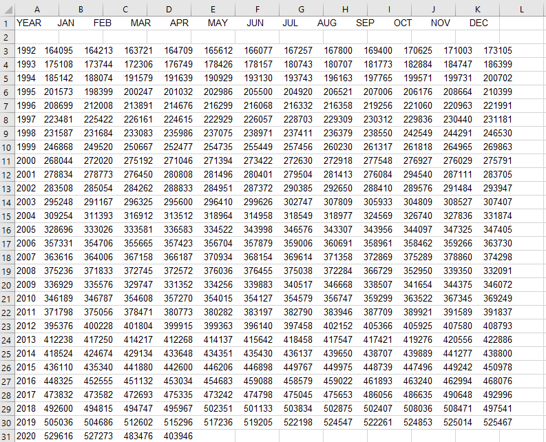
Let’s start with the first step, and that’s to get the data into Excel. It’s in text, but the information is workable since it’s in the format of a table. I’m not going to copy the seasonal factors, I just want the raw, unadjusted sales numbers. To get the data into Excel, I’ll just highlight the sales data, copy it, and then paste it into a blank Excel sheet. Here’s how it looks:

Raw data.

The first thing that needs to be fixed is that everything is in column A. The data as it is won’t be useful for data analysis and needs to be cleaned up before it would make sense to try and transpose it.

Use text to columns to spread data across multiple columns

In Excel, there’s a Text to Columns button right on the Data tab that will help you to quickly and easily spread the data onto many columns. In our example, select column A and click on this button or something that looks similar to it if you’ve got an older version of Excel:

Text to columns button.

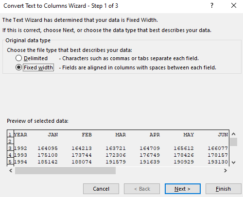
You’ll then see an option for how you want to break out the data. The default is Fixed Width:

Text to Column Wizard step 1.

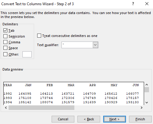
However, that’s not an ideal way to split the data and it rarely ever is. Unless the data is always the same length it won’t be very useful. At best, it’ll be time-consuming to get the output in the format that you’re after. Instead, change the option to Delimited. Click on Next, and then you’ll see various options for splitting the data:

Text to Column Wizard step 2.

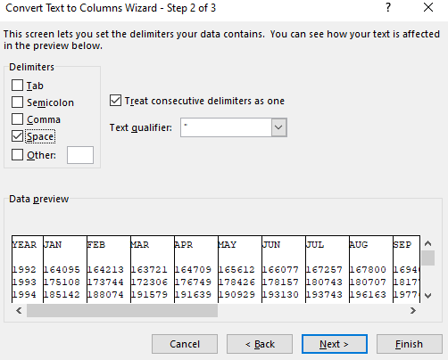
The data isn’t separated by a semicolon, comma, or any other distinctive character. There is, however, a space between each amount. That’s why we’ll want to unselect Tab and tick off the box for Space instead. We see a preview of how the data will be separated, which looks to be what we’re after:

Text to Column Wizard step 2.

At this point we can just click the Finish button and our output will now look like this:

Output after text to columns.

Now we’ve got data that’s much more usable as every number is in its own individual cell. The one thing we’ll want to do before we get to transposing it is to get rid of row 2. The blank row effectively separates the headers from the data, and that’s not ideal.

Next up, let’s get to the actual transposing part.

Transposing the excel data

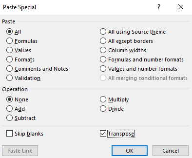
By transposing data, you’re flipping the rows and columns around. And to do that is pretty straightforward. First, copy the data, including the headers, and then click on a blank cell — I’m going to pick O1. Then, right-click and select Paste Special. There, you’ll see an option at the bottom that says Transpose:

Paste special options

Then your data will be flipped, or transposed. You can also select Transpose right from the Paste Special menu and select the icon from there. You can also use shortcut keys S and T to select the menu and then select the transpose button.

Now the data looks like this:

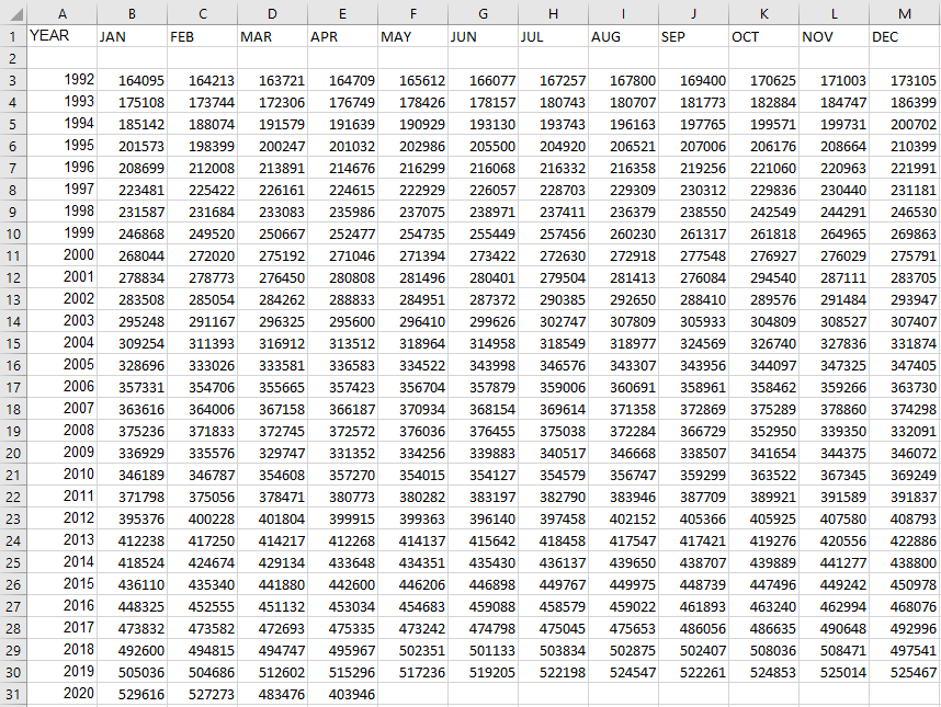
Data after it has been transposed.

The years are now spread across the columns while the months are going down the rows.

Ultimately, whichever way you want to see the data comes down to personal preference. And by transposing it, you can change the view easily to make that happen.


If you liked this post on how to make a transpose data in Excel, please give this site a like on Facebook and also be sure to check out some of the many templates that we have available for download. You can also follow us on Twitter and YouTube.
filterpicture1

How to Filter in Excel

If you’ve got a large data set, you know how important it is to be able to filter that data quickly and easily. Knowing how to filter efficiently in Excel can make it easy to not just pull up the data you need, but to also run calculations. Below, I’ll show you multiple ways that you can filter data.

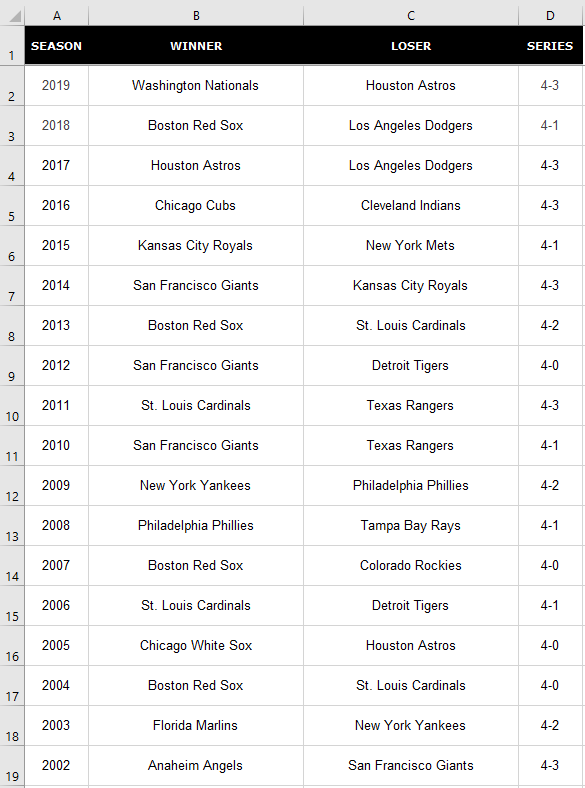
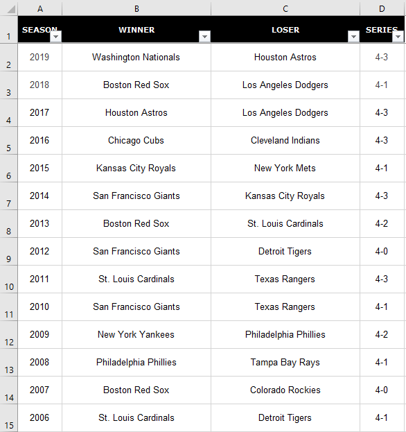
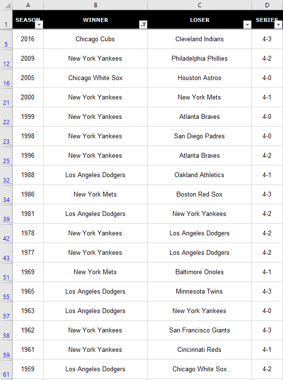
For this example, I’m going to use a list of all the MLB World Series champions and runners-up.

World Series champions and runners up.

Using the auto filter

A quick way to filter the data is by using Excel’s auto filter. To enable it, click anywhere on the data set and click on Filter button from the Data section:

Filter button on the Data tab.

Clicking the button will create drop-down buttons that you can now use to filter the data with:

Data table with filters enabled in the headers.

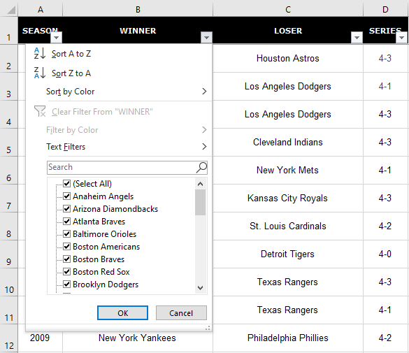
Suppose I wanted to see all the times that the New York Yankees have won. To do that, I would click on the drop-down button in the Winner column, where I’d now see all these options:

Filter options available after clicking on a drop-down.

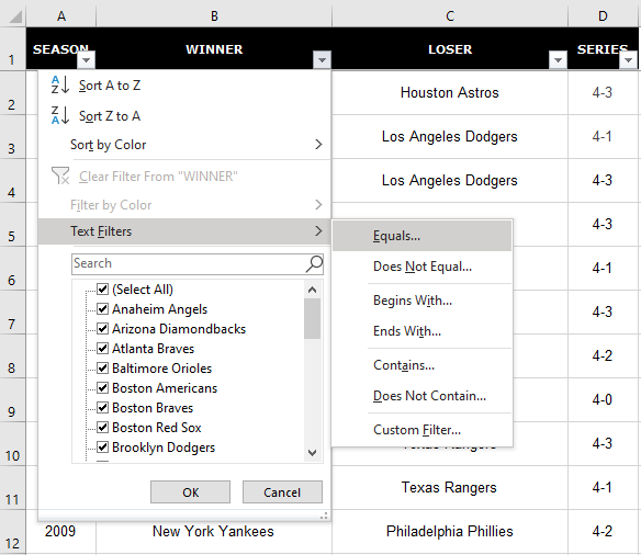
Filtering in Excel can be as easy or complicated as you want it to be. You’ll notice there’s even an option to Filter by Color that’s been greyed out since I don’t have any colors in my data set. If I click on the Text Filter option, I’ll have more options to choose from. I can look for partial matches and I can select an exact match as well:

Selecting equals as the text filter option.

In the following screen, I’ll enter in New York Yankees as my search term:

Selecting a criteria that matches only New York Yankees.

I can also have multiple criteria. For instance, I could say I want to see any victories by the New York Mets as well. In that case I could just enter another criteria and enter their name. However, there’as an even easier way to do that.

Although in the criteria, equals is selected, I can change that by clicking on the drop-down, and there I’ll have more choices:

Selecting filter criteria where the value just contains New York.

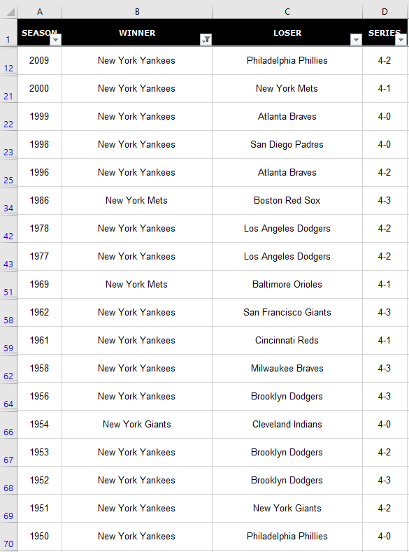
I can select contains and just change the search criteria to New York. So even though I selected equals as my initial match criteria, I don’t have to worry about sticking to it. When I click OK, I now see my list of titles won by any team that had ‘New York’ in their name:

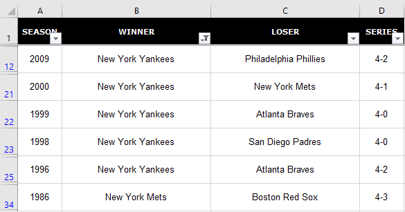
Filtered list showing any time a team from New York has won.

Not only do we have the Mets and Yankees on this list, but there’s also the New York Giants.

You’ll notice that the row numbers on the left are now in blue. This is how you can tell that your data is filtered. And so if you’re looking at your data set one day wondering why you’re missing information, have a look at the row numbers, as they may tell you the data’s filtered. If you want to unfilter the data, go back to the Filter button and click it again. Then your data set will be unfiltered and the drop-downs will be gone.

What you can also do is select the individual drop-down and clear the filter. You can tell which column has a filter in place by looking at the drop-down. In the Winner tab, the button shows a filter icon:

Drop down shows a filter icon, indicating the column has been filtered.

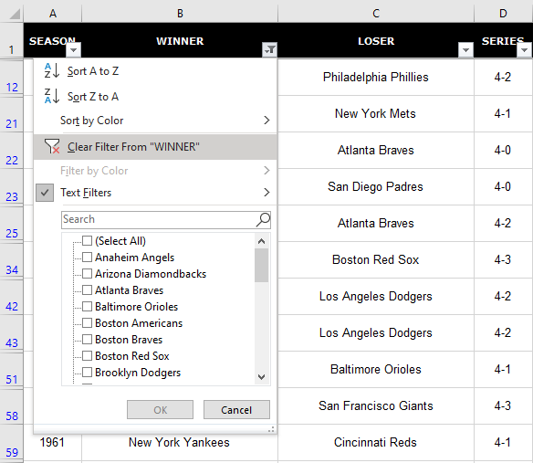
Clicking on that drop-down I’ll have the option to eliminate the filter:

Clearing a filter.

Clicking the Clear Filter From “WINNER” button will now reset the filter and keep the drop-down buttons in place.

Filter using selections

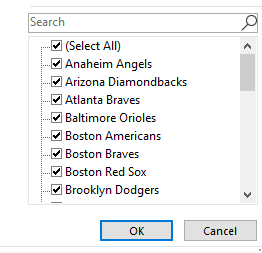
Using the text filter isn’t optimal because on newer version of Excel you see the list of items that you can choose from:

Choosing from the values list.

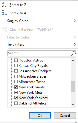
If I uncheck Select All and then scroll down to the New York teams and select them, I’ll arrive at the same result as if I did the text filter earlier:

Checking off the values to filter.

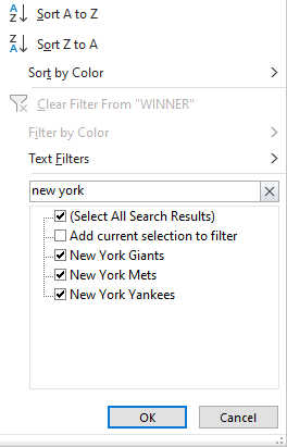
However, even this isn’t optimal. If I’m looking for a partial match, then I can just type in ‘New York’ in the search field and it’ll get the same selections:

Filtering by using the search field.

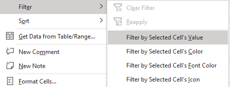
There’s another less common way that you can filter data. If you’re just looking for one match, you can right-click on the value that you want to filter. Then, right-click on it and click Filter by Cell’s Value:

Filtering by selection.

With this method, the drop-downs in the headers don’t have to be enabled. Once you run this filter, they will be there, however.

Filtering multiple combinations

It’s easy to filter when the names are similar. But if I wanted to filter the data for anytime a team from New York, Chicago, or Los Angeles has won, then it gets a bit trickier. One method would be to go back to the text filters and run multiple filters. But that’s an antiquated way of doing it. However, if you’re running an older version of Excel, that may be your only option.

If you can search through the filter, then there’s an easier way for you to do this. First, let’s go back to searching for ‘New York’ in the filter. We’ll again have all the New York teams in the list.

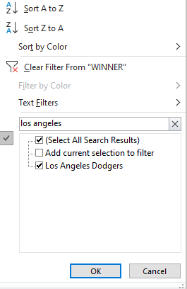
Next, let’s go back to the drop-down and search again. This time for ‘Los Angeles’ but before clicking OK, we’ll want to click off the box that says Add current selection to filter:

Add current selection to filter checkbox.

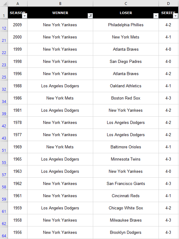
By default, this option isn’t checked. If I were to just click OK, the filter would be a list of Los Angeles teams only. But by checking off that box first and then clicking OK, I now have a list that contains both Los Angeles and New York:

Multiple cities filtered.

After repeating the process for Chicago I’ve now got all three cities in my list without having to go through the text filter:

All three cities filtered on the list.

Use subtotals to make your filters even more useful

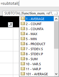
If I wanted to run a quick tally to see how many of the teams I’ve filtered have won a championship, I could use a COUNTIF function and enter their names. But if you want something more flexible where you can quickly run the filters as I’ve done above and see how many teams are in that list, you can use the SUBTOTAL function. The function takes in an argument for what type of calculation you want to do.

Arguments listed in the subtotal function.

Now, since this data isn’t numeric, I’m going to use a COUNTA function, which is function number 3. For the range, I can use any column since it doesn’t matter which one I’m counting. But I will use range A2:A1000 because I don’t want to include the header in my total. Here’s how my formula looks like:

Subtotal formula counting all the entries that have been filtered.

I could also use the MAX function to see the last time one of the teams I’ve selected has won. I’ll put that directly below the other formula:

Using multiple subtotals in a filter.

Now, if I were to re-filter this data, this time, only for New York, my subtotals will automatically update:

The benefit of using the SUBTOTAL function is your data updates along with your filters. If you want the data to be static and not change, that’s when a regular COUNTIF function would be more appropriate.


If you liked this post on how to filter in Excel, please give this site a like on Facebook and also be sure to check out some of the many templates that we have available for download. You can also follow us on Twitter and YouTube.

matrix-1027571_1280

How to Combine Two Columns in Excel

If you’ve inherited or downloaded a data set, you know that sometimes you’ll need to combine data together to make it in the format that you want. A good example is a list of addresses where you may have the street information in one column and the zip or postal codes in another column. To get all the information in one cell would require combining the information. Below, I’ll show you multiples ways of how you can combine two or more columns in Excel.

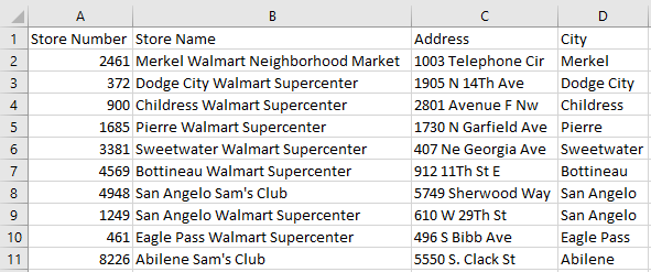
My data set for this example includes some sample address information on Sam’s Club and Walmart locations in the U.S. :

Address information on Walmart and Sam's Club locations in the U.S.

Using the ampersand to combine columns together

The easiest way is to join the cells through a simple formula. The easiest way to do so is by using the ampersand (&). In column D below, I’ve joined the cells and in column E is the formula that I’ve used:

Combining two columns together in Excel using the ampersand.

This gets the job done but you’ll notice a small issue: there isn’t a space between the information. that makes the data a bit messy and it’s probably not what you want. But it’s an easy fix. It can be addressed by adding another ampersand between the cells and add open quotes ” ” to add a space. This is how my spreadsheet looks after I’ve made those changes:

Combining multiple columns in Excel using the ampersand and adding a space.

This can be expanded to more than just two columns. If I wanted to add the store name field (column A) into the mix, then it’s just simple as adding another ampersand for the field and another one for another extra space. Here’s how the data looks like all three columns joined together:

Combining three columns together in Excel using the ampersand and spaces.

This can start to become a bit cumbersome as you add more fields into one cell. An alternative way that you may find easier if you’re working with several columns is using the CONCATENATE function.

Using the CONCATENATE function

The CONCATENATE function works very similar to how the ampersand. However, it’s a bit cleaner in that you don’t have several ampersands in your formula. If you wanted to group cells A2, B2, and C2, your formula would look like this:

=CONCATENATE(A2,B2,C2)

If you want a space to be included between each of those fields, then it looks like this:

=CONCATENATE(A2,” “,B2,” “,C2)

Here’s how that would look if I applied it to my existing data set:

Combining three columns in Excel using the concatenate function.

You can use commas to separate the data if you prefer and in that case, you would just use “,” instead of an empty quote. You can also add extra spaces in between quotes to space out your data even further.

But whether you choose to use the ampersand or the CONCATENATE function just comes down to preference. Either approach can get the job done.


If you liked this post on how to combine cells in excel, please give this site a like on Facebook and also be sure to check out some of the many templates that we have available for download. You can also follow us on Twitter and YouTube.
webdesign-3411373_640

3 Reasons Why You Should Always Save Excel Templates as .xltx or .xltm

If you’ve spent the time to create a template in Excel, it’s important to save it in the right format to help protect your work. While the temptation may be to just save it as the default .xlsx or.xlsm format, you’re best off saving it in the correct template format – .xltx or .xltm, and here’s why:

1. You avoid easily overwriting the file

One of the biggest mistakes you can make with a template is not backing it up. As much as you can test a template to make it as error-proof as possible, someone usually will find a way to make it not work the way it was intended. If someone uses the live template file then that’s just asking for trouble. Once data is entered on the file and things are moved around, if something is not working at a later point in time it’s hard to go back and try and figure out what went wrong, especially if the structure or file was changed in some way.
One way I normally mitigate this is by saving the template somewhere else and have someone use a copy of it. If something has gone terribly wrong and formulas have been altered, it’s a lot easier to copy the data back into something that you know was working (the file that was backed up) than it is try and troubleshoot on a modified file where you’re unsure as to what has changed.

Saving it as a template file (.xltx or .xltm – for templates with macros), however, will allow you to mitigate the potential for someone to save over the template by accident. By saving it as one of these formats, when a user opens the template file it will automatically change the name to add a number to it and when they go to save it won’t save as a template file (unless they manually change it). While a user can still technically save over the template file, it’ll take some work to do so. In all likelihood, the user will end up saving it as a non-template file. Either way, you’ll still probably want to save a backup file somewhere else, but the risk of being overwritten should be minimized this way.

2. It makes it easy to find your templates on your computer

If you have your Excel files, including templates, in one folder, it becomes easier to sort and identify the templates by just looking for those that end in .xltx and .xltm. What you can do is sort by file type or when you go to open a file select the type of file you’re looking for. This will help avoid opening the wrong file.

If your files aren’t all in one location, you could also do a search of files ending with .xlt across a range of folders to help find all your templates. This could make it easier than to add the word ‘template’ into every one of your templates.

3. Easy access for users

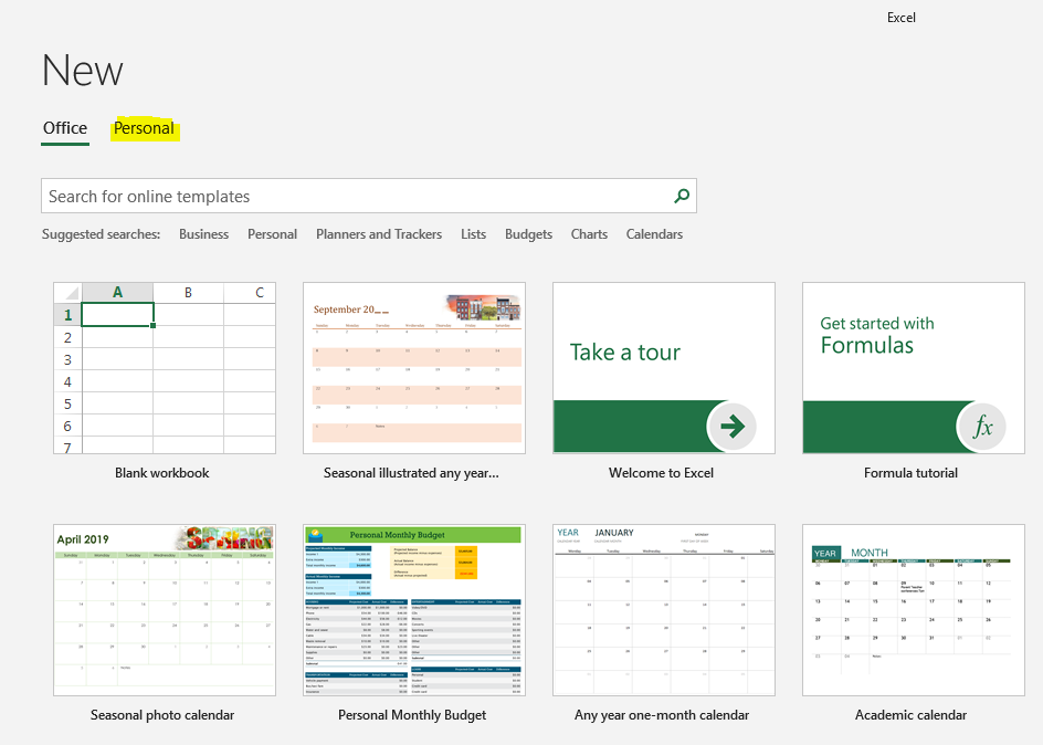
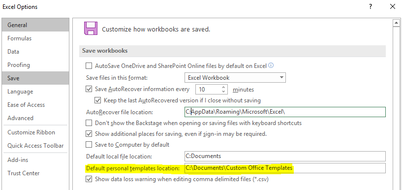
By default, when you go to save a .xltx or .xltm file, Excel will select the templates folder. You don’t have to save your files there, but by doing so your templates will now show up when a user goes to create a new file and looks for templates. Your saved templates will be available by selecting the Personal section:

By being able to access the templates when creating a new file, a user doesn’t have to worry about finding the location of a template. If you don’t want to use the default location that Microsoft has assigned for templates, you can change the folder in the Excel options under the Save section:

This way you can also have all your templates in a shared location among many users. The user would simply need to change these settings to direct Excel to the correct folder.

money-2696219_640

How to Calculate CAGR in Excel

When you’re doing financial analysis, it’s helpful to add some context to growth numbers. That’s where using a Compounded Annual Growth Rate (CAGR) is very useful. Rather than saying a company has grown 50% over 10 years, you could say instead that they’ve grown by an average of 4.1% every year. It also gives you a percentage to use going forward if you need to forecast what you expect next year’s growth to be since you’ll have a starting point. The CAGR effectively tells you what the average growth rate has been during that period of time. It doesn’t mean that it’s grown every year by that rate, but that on average, it has risen by that amount. Below, I’ll go over how to calculate CAGR in Excel.

Using Amazon as an example

To calculate CAGR what you need to know are just two things: the total growth and the duration of time. Let’s use Amazon’s sales as an example. In 2018, total revenues for the year reached $233 billion. Back in 2010, the company had $34 billion in sales, meaning that Amazon’s revenues have grown by 585% during that time. Impressive, no doubt, but it doesn’t tell us how well it’s typically done on a yearly basis. This is where we calculate CAGR to help determine what the average growth was over that time.

From 2010 to 2018, that’s eight years that it took for sales to grow by 585%. To calculate CAGR, we use the following equation:

(Current Year Amount / Base Year Amount) ^ ( 1 / # of Years)

In the Amazon calculation, it would look as follows:

(233/34) ^ (1/8) – 1 = 27%

What this tells us is that Amazon for the past eight years has averaged an annual growth rate of around 27.2%. There’s an easy way we can prove this out. Starting with our base year of 2010, take the sales amount of $34 billion and multiply it by (1 + growth rate) each and every year. Here is how the level of growth looks like year over year:

YearPrior Year
Revenue
GrowthCurrent Year
Revenue
2010 $34, 000
2011 $34,000 27.2% $43,248
2012 $43,248 27.2% $55,011
2013 $55,011 27.2% $69,973
2014 $69,973 27.2% $89,006
2015 $89,006 27.2% $113,215
2016 $113,215 27.2% $144,008
2017 $144,008 27.2% $183,177
2018 $183,177 27.2% $233,000

As you can see, if we assume a 27.2% growth rate each and every year, we arrive to the same end value. Although Amazon did not grow at this consistent of a pace, using CAGR helps to average the results over a period of time.

Whether you’re looking at sales, dividends, or any other kind of growth, using CAGR can be a very useful tool in putting into context just how the strong the rate of growth was.

Using CAGR to help forecast

Having CAGR is also useful if we want to forecast out future sales. Let’s assume that Amazon will have a more modest rate of growth for the next 10 years. That rather than a CAGR of 27.2%, it’ll be closer to 20% instead. Now, we can create a forecast around that and assume that sales will grow by 20% each year (on average) for the next 10. Our forecast would look as follows:

YearPrior Year
Revenue
GrowthProjected
Revenue
2019$233,000 20%$279,600
2020$279,600 20%$335,520
2021$335,520 20%$402,624
2022$402,624 20%$483,149
2023$483,149 20%$579,779
2024$579,779 20%$695,734
2025$695,734 20%$834,881
2026$834,881 20%$1,001,857
2027$1,001,857 20%$1,202,229
2028$1,202,229 20%$1,442,675

To prove this out, what we can do is the following: 233,000 x (1.20^10) = 1,442,675

Based on these projections, we would expect amazon to hit the one trillion dollar mark in sales by the end of 2026. Maintaining a CAGR of 20%, however, will be difficult, even for a company like Amazon. Although all it takes is some big acquisitions and it will be well on its way!

If you don’t want to calculate CAGR on your own, you can use our free online calculator!


If you liked this post on How to Calculate CAGR in Excel, please give this site a like on Facebook and also be sure to check out some of the many templates that we have available for download. You can also follow us on Twitter and YouTube.