One of the most frustrating things that can happen to the spreadsheet you’ve spent hours or days on is when someone overrides a formula or a cell with important information. That why it’s important for people making and designing spreadsheets to be familiar with how to lock cells in Excel. It’s not a difficult thing to do and it can save you a lot of headaches down the road. There are two ways you can go about doing it. I’ll start with the approach that should work even on older versions of Excel:
Step 1: Unlock all the cells
By default, Excel sets that status of every cell to locked. However, until you actually protect a sheet none of that goes into effect. But you’ll actually want to undo that. The first thing you should do is select all the cells (CTRL+A) in your sheet and then go into Format Cells (CTRL+1). From there, go into the Protection tab where you’ll see this:
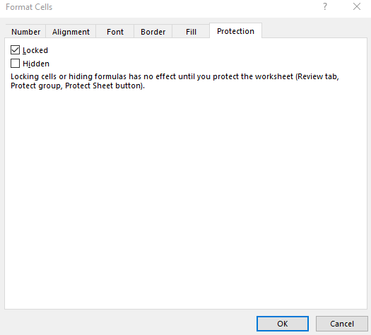
Untick the ‘Locked’ box and this will leave all the cells unlocked. It sounds like the opposite of what you want to do. However, it’s easier to unlock everything and then re-lock the cells you really need locked. Doing the reverse is going to be more time-consuming.
Step 2: Select the cells you want to protect and then lock them
Now, its time to select the cells that you want to lock. Formulas, any sort of rate schedules or information that shouldn’t be changed are things you’ll want to identify. Once you’ve selected them all, you can go back into Format Cells and this time you can re-check the box to have them locked. If any of these cells contain formulas that you don’t want people to see, you can also tick off the Hidden box. Doing this will prevent anything from showing up in the formula bar when someone looks at one of these cells.
Step 3: Lock your worksheet
Even though you’ve already selected which cells you want to be protected, nothing’s technically happened just yet. What you still have to do is lock the worksheet itself. On the Review tab, you’ll have a button to Protect Sheet. Click on that, and you’ll have the following options to choose from:
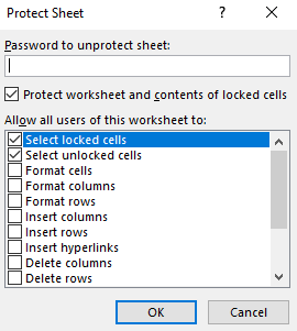
First thing’s first, you’ll want to put a password in. Otherwise, there’s really no point in protecting these cells if someone can just unlock the sheet without any password.
By default, Excel selects the first to options when protecting cells, allowing users to select both locked and unlocked cells. However, you can untick the locked cells if you don’t want them to be able to even select locked cells. If your goal is just to protect cells, these two options should suffice. But you can also restrict formatting cells, inserting and deleting rows as well.
Once you click OK, if you’ve entered a password, you’ll be prompted to re-enter it again to confirm it. Now your cells are protected. If you attempt to change the value on any of them you’ll get the following error message:

If you want to be able to change those cells, you’ll now have to go back to the Review tab and click on Unprotect Sheet. There, you’ll be asked for a password if you’ve entered one.
Optional step: highlight the cells you plan to lock
To prevent frustrating your users, you may want to take an additional step and highlight the cells that they either should or shouldn’t enter values in. This will avoid them getting frustrated with error messages popping up when they try and make changes. Highlight cells can make it a lot easier for users to identify which cells they should edit.
Tip: here’s a quick way to to find all your formulas
If you don’t want to hunt down all the formulas in your sheet that you want to protect, the good news is it’s easy to find them. You can use CTRL+~ to toggle showing formulas or values on your worksheet. However, there’s an even easier way to select all your formulas. By pressing F5 you’ll get the Go To box:
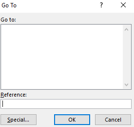
Click on Special (this is greyed out once you’ve locked the worksheet, so you’ll want to do this beforehand). Then, click on Formulas in the next menu:
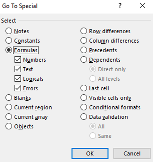
Click OK and now all your formulas will be selected. From here, you can go to the Format Cells options and make sure they’re locked or hidden.
What if you’ve made a mistake and protected the wrong cells?
If you need to make a correction to which cells you’ve selected, all you need to do is to unprotect the sheet. Then repeat steps 1-3. But you may notice something odd when you go back to unlock all the cells:
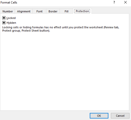
This is how the checkboxes will show up if not all cells are locked and not all cells are hidden. You’ll only see the boxes blank or ticked off if all the cells have the same values (e.g. protected or hidden). Clicking once on each of these text boxes will turn them into checkmarks:

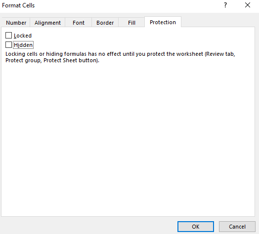
If you were to click OK then all the cells would be locked and hidden. Clicking these checkboxes an additional time will make them all unlocked and unhidden (but not until you protect the worksheet):
The alternative approach: Protect cells in Excel using the Allow Edit Ranges option
Below, I’ll show you another way how to lock cells in Excel that doesn’t require unlocking and re-locking cells. Rather than following steps 1-3 what you can first do is use the Allow Edit Ranges button on the Review tab. Pressing that button will give you the following options:
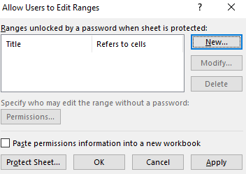
From here, you can click on the New button. Next, select a range that you want users to enter data on:
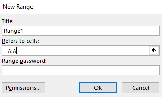
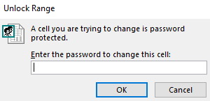
In this example, I’ve set a name of Range1 to everything in column A. I’ve also put no password for this range. Now, if I go to protect my entire worksheet, I can still edit any cell in column A (regardless of it is set to locked or not). If I had added a password for that range, I’d be prompted to enter it before gaining access to the range:
You also have the option to designate certain users who don’t need a password to edit the range. You can do this by clicking on the Permissions button:
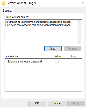
What’s also convenient about the Allow Edit Ranges feature is that you also can protect the sheet right from its options.
Which method should you use?
Ultimately, both methods can help you protect your cells and formulas in Excel. If your worksheet is very structured and there are only certain places where users should make changes, then using the Allow Edit Ranges approach probably makes a lot more sense.
If, however, most of your cells should be editable and there are only a few cells that you need to lock or they’re spread out all over the place, then the first method may be preferable.
Either approach can work and it may just come down to your personal preference on how to lock cells in Excel.
Adding additional controls—locking down the workbook
If you want to take things a bit further and prevent people from modifying, viewing, or deleting worksheets, what you can do is protect your workbook as well. This is a simpler than how to lock cells in Excel and all that you need do here is just click on the Protect Workbook button and put a password on your entire workbook. Doing this will prevent users from renaming, moving, deleting, or hiding worksheets.
If you’d just prefer users don’t see certain worksheets and don’t even see that they’re there, you may want to consider using VBA to hide them without having to lock your entire workbook down. In some cases, locking a workbook may work well at preventing worksheet changes, but it’s an all-or-nothing approach: you can’t pick and choose which worksheets they can change — that’s where VBA can help.
If you liked this post on how to how to lock cells in Excel, please give this site a like on Facebook and also be sure to check out some of the many templates that we have available for download. You can also follow us on Twitter and YouTube.

