When working with a pivot table, you determine a data source to use for that table. But what if later you add rows or columns? You’ll normally have to change the data source to include the updated range, otherwise your pivot table isn’t including your changes. Unless you use a named range.
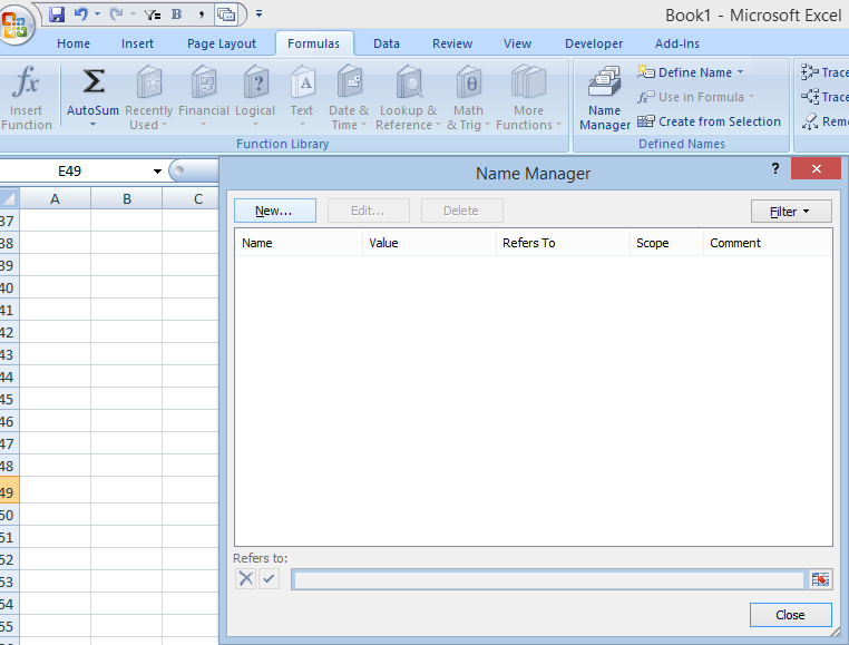
First, select the Name Manager under the Formulas tab and click on New
However, instead of selecting all the data, I’ll use the offset formula.
The OFFSET function allows you to specify the size of your data set. The formula below will keep the range equal to all the nonblank rows and cells starting from cell A1:
=OFFSET(Sheet1!$A$1,0,0,counta(Sheet1!$A:$A),counta(Sheet1!$1:$1))
This is the first cell of your data source
This is the first column of your data source
This is the first row of your data source
Once you’ve created a new name for your data set, put the formula above in the Refers to field and press OK:
Now you’ve created your custom, auto-updating range. All you need to do now is when creating a pivot table (or changing its data source), put in the named range.
Note this will not work properly if you have gaps in your columns or rows. The COUNTA function counts how many non-blank cells are within the range. So you could manually override the formulas if need be, but that would defeat the point of this post.
But if you follow the above steps and use the formula above, your pivot table will automatically be updated with any new rows or columns you add to it. All you’ll have to do is refresh the pivot table. And because the offset formula forces the range to change, that will automatically happen in the pivot table as well.


Add a Comment
You must be logged in to post a comment