How to Unpivot Data in Excel

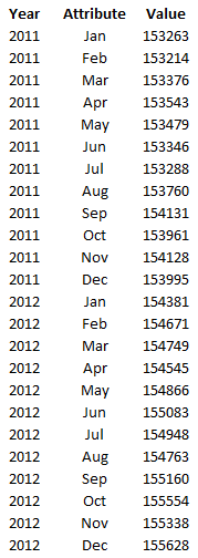
Using pivot tables to summarize data can be a great way to display information quickly and total everything up. However, in some cases, data that you download is already in what you might call a pivot table format where it is summarized and you want to put it in more of a tabular format. In this post, I’ll show you how to unpivot data in Excel where you can turn a table like this:

into this:

Unpivot using Power Query

Rather than copying and pasting data into a tabular format and doing the process manually, you can just use Power Query to do it for you, all in a matter of seconds. First thing’s first, you need to get your summarized data into Power Query. To do that, click on one of the cells in the table and on the Data tab, click on the From Sheet button in the Get & Transform Data section:

Then, click OK on the default range and then the next screen will be Power Query:

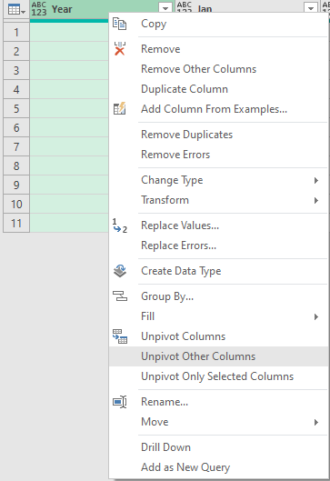
The key to making the unpivot work correctly is to determine which column(s) you don’t want to unpivot. In this case, it is only the Year field as I want to have the years listed out. With the Year column selected, I right-click on the header and select Unpivot Other Columns:

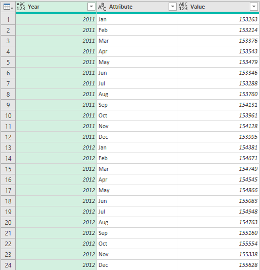
After clicking on that, the data is unpivoted and now it is in tabular format:

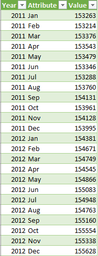
All that is left now is to press the Close & Load button in Power Query, which will then populate the data back into Excel:

You can repeat these steps for other, similar summarizes should you need to unpivot data.

If you liked this post on How to Unpivot Data in Excel, please give this site a like on Facebook and also be sure to check out some of the many templates that we have available for download. You can also follow us on Twitter and YouTube.