How to Do a Picture Lookup in Excel

A lookup is one of the more common things you can do in Excel. Whether you’re using VLOOKUP, a combination of INDEX and MATCH, or the new XLOOKUP, there are no shortage of ways to accomplish it. However, in this post, I’ll go over how you can do a lookup that involves pulling in a picture. It’s a bit more complicated to set up but once you’ve figured it out, it should be a breeze.

Step 1: Create a table of the images you would like to use

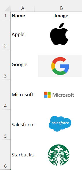
I’m going to create a tab for images that has two columns — one for the name of the image, while the other will hold the image itself. I’m going to make the rows wide, with a height of 60 just to make sure the cell can fit the entire image. In this example, I’m using some popular corporate logos:

Step 2: Setup the named ranges

Next, I’ll create named ranges in column B that match the values in column A. In the example above I don’t have any spaces but if I did, I would replace them with an underscore to make sure there are no gaps. In addition to creating a named range for each individual logo, I will also create a named range that contains all the values in column A. This way, I can use this as a dropdown later on to select which logo I want to select.

I’ll create a named range called ‘Companies’ for these options. When using data validation, I’ll just enter the following as my list options:

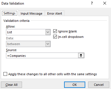
I’ll add this on to another sheet. My selection here will determine which image to pull.

Step 3: Creating another image for the lookup

I also need to create a picture that will pull the desired image. To do this, I can just copy any one of the images I inserted in the first step.

Step 4: Creating a named range for the selection

I’m going to create another named range, this time, I won’t be selecting a cell but I will go through the Formulas tab and select Name Manager where I’ll see all the named ranges I have set up thus far:

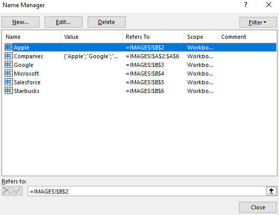
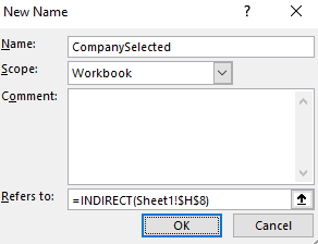
Click on the New button. And here, I’ll need to use the INDIRECT function to reference the cell that contains the company value that was selected through the dropdown. In my example, that is cell H8. My named range, which I’ll call, ‘CompanySelected’ will look as follows:

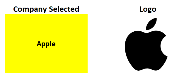
Now, for the picture that is acting as your lookup, select it, and set the cell equal to the named range of ‘CompanySelected’ :

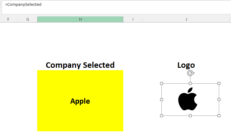
I can adjust the size as large as necessary. And now, when I change my dropdown option, the image will automatically update:

If you liked this post on How to Do a Picture Lookup in Excel, please give this site a like on Facebook and also be sure to check out some of the many templates that we have available for download. You can also follow us on Twitter and YouTube.