Google Sheets makes it easy to pull in data from the internet, including stock prices. An advantage it has over Excel’s StockHistory function is that it can pull prices even before the trading day has finished. This gives users access to more up-to-date information. Plus, it’s easy to track not just one or two stock prices in Google Sheets but even hundreds.
How to pull in a stock price for a ticker symbol in Google Sheets
Using the GOOGLEFINANCE function, you can quickly pull in a stock price easily. Here are the main components of the function:
- Ticker
- Attribute. Below are the attributes you can use for stocks:
- “price”: current price, up to 20 minutes delayed.
- “priceopen”: the opening price.
- “high”: the current day high.
- “low”: the current day low.
- “volume”: the current day’s volume.
- “marketcap”: the stock’s current market cap.
- “tradetime”: the time the last trade was made.
- “datadelay”: how delayed the real-time data is.
- “volumeavg”: the stock’s average trading volume.
- “pe”: the price-to-earnings ratio.
- “eps”: the most recent earnings per share.
- “high52”: the stock’s 52-week high.
- “low52′: the stock’s 52-week low.
- “change”: the change in stock price from the previous day’s close.
- “changepct”: the percentage change in price from the previous day’s close.
- “beta”: the stock’s beta value.
- “closeyest”: the previous day’s closing price.
- “shares”: the number of shares outstanding.
- “currency”: the stock’s currency
- Start Date
- End Date
- Interval
You don’t, however, need to fill in all of the arguments. For example, the following formula only uses the ticker and the attribute field and it will pull in Amazon’s current stock price:
=GOOGLEFINANCE(“AMZN”,”price”)
If you want to pull in Amazon’s stock price for the first trading day of the year, you could use the following formula:
=GOOGLEFINANCE(“AMZN”,”price”,”1/1/2024″)
This will return the following table:

Although January 1 was not a trading day, the formula automatically gets the data for the next trading day. If you just want to get the closing price and don’t want the rest of the table, you can nest this formula within the INDEX function as follows:
=INDEX(GOOGLEFINANCE(“AMZN”,”price”,”1/1/2024″),2,2)
Since we are getting the second column and the second row, it will only retrieve the closing price for that day. This method works when you are just pulling in the stock price for a single date.
Adding a prefix for exchanges
If you want to track a lot of stocks, the one thing you may inevitably run into is a situation where Google Sheets doesn’t correctly identify your stock ticker. If, for example, you want to pull in a stock from a different exchange, entering just the ticker symbol alone won’t be enough. If I wanted to pull in the price for Air Canada stock, which has a ticker symbol AC on the Toronto Stock Exchange (TSX), this formula won’t work:
=GOOGLEFINANCE(“AC”,”price”)
Instead, that formula will return the value for Associated Capital Group, which trades on the NYSE. Google Sheets effectively takes its best guess as to which ticker you want to pull in. But as you can imagine, it may get it wrong if you have a symbol which is active on multiple exchanges.
To get around this, you can incorporate an indicator for the exchange. For the TSX, it’s TSE. If you’re not sure which one to use, go to the Google Finance website and look for the stock you want, and take note of the code for the exchange:

To ensure the GOOGLEFINANCE function is retrieving the correct stock, I can adjust my formula as follows:
=GOOGLEFINANCE(“TSE:AC”,”price”)
You can follow the same methodology for other stocks and exchanges.
Creating a template to track hundreds of stocks
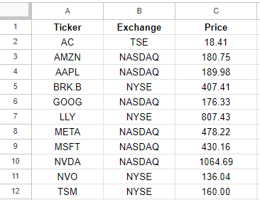
To create a template to help you track stocks in Google Sheets, all you really need are a few fields. One for the ticker, one for the exchange, plus one for the stock price. I’ll also add one for the % change. This can help you build out a dashboard.
If I have my tickers in column A and the exchange code in column B, I can combine the values to create a dynamic formula which will update based on those combinations. This way, I can avoid having to hardcode the individual stock tickers. Here’s how that formula would look:
=GOOGLEFINANCE(B2&”:”&A2,”price”)
The key is to combine those values and separate them with a colon in-between, so that the format is exchange:ticker. Now, when I create my template, I can copy that formula down and it will pull in stock prices which aren’t based solely on just the stock ticker:

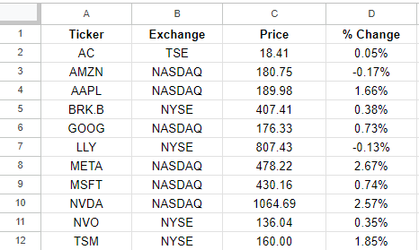
Let’s extend this a bit further and now also include the percent change from the previous day. If I want to format it as a percentage, I need to make sure I divide the value by 100:
=GOOGLEFINANCE(B2&”:”&A2,”changepct”)/100
And now I can display both the stock price and the percent change from the previous day:

You can copy these formulas down hundreds of rows, making it possible to track as many stocks as you need in Google Sheets.
If you like this post on How to Track Hundreds of Stocks in Google Sheets, please give this site a like on Facebook and also be sure to check out some of the many templates that we have available for download. You can also follow me on Twitter and YouTube. Also, please consider buying me a coffee if you find my website helpful and would like to support it.

