
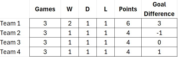
If you’re tracking standings in Excel, you know it can be challenging to ensure that you have your rankings setup correctly, especially when factoring in multiple criteria. Ranking values based on a single column or field isn’t complex, but when you start to factor in multiple conditions, it can get a little bit more complicated. Here’s a scenario I’ll attempt to solve where multiple teams have the same number of points, but where their goal difference isn’t the same:
By using an additional criteria as a tiebreaker, you can ensure you rank the teams properly. But how do you setup the formula, and what if you also want to factor in more columns and use a method which can be used for more complex situations? That’s what I’ll go over in this post.
Using the Rank function
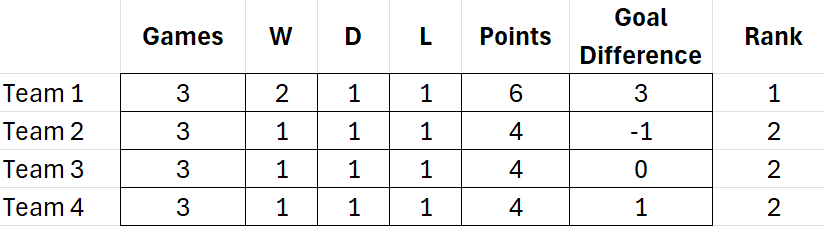
If you were to rank these teams based on points, you would use the RANK function. You would use the value in the points field and rank it based on those values. If my first value is in F2 and the range for the points field is F2:F5, my formula would be as follows:
=RANK(F2,$F$2:$F$5)
The limitation of this method is that it will result in repeating values since multiple teams have 4 points:
How to use multiple criteria in your ranking calculations
The RANK function only allows us to base the calculation on a single field. But there is a way we can still rank the values based on multiple fields. This involves using multiple functions, and fractions. Assuming the key criteria is points, then the current formula can be kept as is. But let’s assume the second criteria is goal differential. Then, we can rank the teams based on this field, but divide the value by a factor of 10. Here’s what the formula would look like assuming goal difference is in column G:
=RANK(G2,$G$2:$G$5)/10
This then gets added to the original formula:
=RANK(F2,$F$2:$F$5)+RANK(G2,$G$2:$G$5)/10
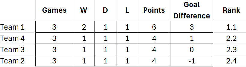
Based on this calculation, now my formula shows an additional decimal point and I can now rank the fields based on a second field:
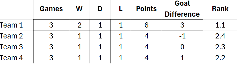
And now I can re-sort the data based on the rank, which correctly tells me that Team 4 is in second place when ranking them based on points, and then goal difference.
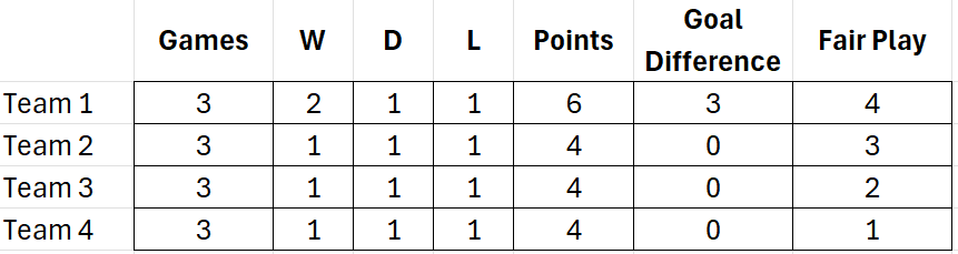
You can extend this logic to more criteria and fields. Let’s assume a more complicated scenario where the goal difference for the tied teams is 0. And instead, it comes down to a third criteria, which is their fair play score:
Assuming Fair Play is in column H, here is my updated ranking calculation:
=RANK(F2,$F$2:$F$5)+RANK(G2,$G$2:$G$5)/10+RANK(H2,$H$2:$H$5)/100
In this situation, Team 2 will have the second-best ranking because it has the best fair play score.
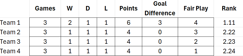
My ranking calculation now has yet another decimal place and another criteria which it can factor into its calculation. You can also adjust the criteria if, suppose, the lowest score for Fair Play is the best. Let’s say the lower the Fair Play score, the better the team should rank. In that case, we can adjust the formula so that we specify the rank should be in ascending order for that last criteria (the default is descending order):
=RANK(F2,$F$2:$F$5)+RANK(G2,$G$2:$G$5)/10+RANK(H2,$H$2:$H$5,1)/100
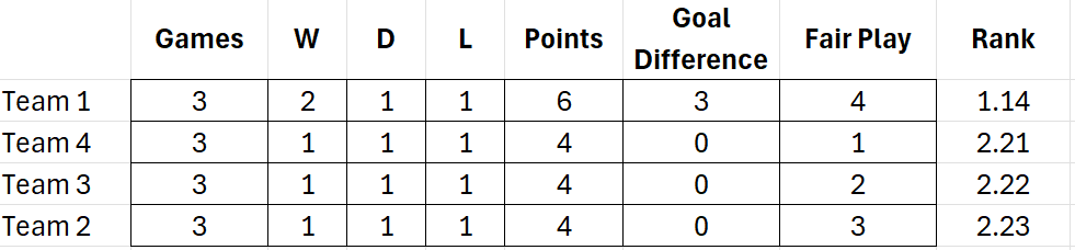
I just needed to add the final argument to the last criteria, setting it to 1. And now when I re-sort the rank, Team 4 gets the second spot:
By setting up your ranking calculation this way, you can have the flexibility of adding more fields and criteria into your ranking. If you want to add another field, simply add it to your formula and divide that value by 1000, and so forth.
If you like this post on How to Break Ties in Excel and Rank with Multiple Criteria, please give this site a like on Facebook and also be sure to check out some of the many templates that we have available for download. You can also follow me on Twitter and YouTube. Also, please consider buying me a coffee if you find my website helpful and would like to support it.