Pivot tables are a powerful feature in Excel that allow users to summarize, analyze, and visualize data. One of the more advanced features of pivot tables is the ability to add calculated fields. Calculated fields enable you to perform calculations on the data within your pivot table without modifying the original dataset. This can be incredibly useful for generating new insights and custom metrics. In this post, I’ll show you how you can take them a step forward and even incorporate IF statements within calculated fields. Here’s the data set that I’m going to use for this example:

How to add calculated fields in a pivot table
To add a calculated field to a pivot table, take the following steps:
1. Convert your data into a Pivot Table.
2. Click on any cell within your Pivot Table to activate the PivotTable Analyze tab on the ribbon.
3. On the PivotTable Analyze tab click on Fields, Items & sets and then select Calculated Field
4. Enter a name for your calculated field in the Name box.
5. Write out the formula you want to use in the Formula box. You can use existing fields (columns) from your dataset by double-clicking on the field names listed in the Fields box.
6. After you’ve completed writing your formula, click Add then press OK. Your calculated field will be added to the PivotTable, typically in the Values area.
How to use an IF statement in your calculated field
One of the more powerful uses of calculated fields is the ability to include conditional logic using an IF statement. This allows you to create dynamic calculations that can change based on the criteria you set. For my pivot table, I just have a list of dates to start with:

Suppose I want to create a calculated field which will show a value if it is profit (i.e. a gain), and a loss field which will show a value when it is negative.
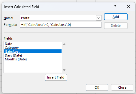
In the formula box, I’ll write an IF statement for my profit field calculation. It will reference the gain/loss field which I already have. If the value is positive, it will retrieve that value, otherwise it will be zero.

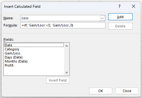
Now, I’ll click on Add and then I’ll setup the Loss field:

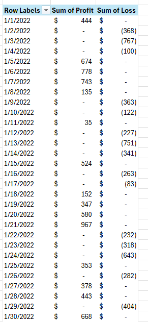
Now when I add these fields to my pivot table, I have one column for the profit values, and one for the losses:

If you like this post on How to Track Income and Expense in a Single Chart, please give this site a like on Facebook and also be sure to check out some of the many templates that we have available for download. You can also follow me on Twitter and YouTube. Also, please consider buying me a coffee if you find my website helpful and would like to support it.

