
Did you know you can create a pivot table in Google Sheets which automatically updates as you add data to it? Remarkably, it’s an easier process than in Excel where you would need a macro or where you might need to right-click on the pivot table and select to refresh the data. Here’s how we can go about creating a pivot table in Google Sheets, and having it automatically update.
Creating a pivot table in Google Sheets
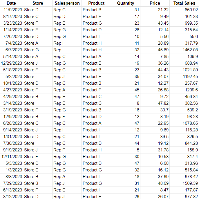
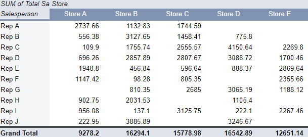
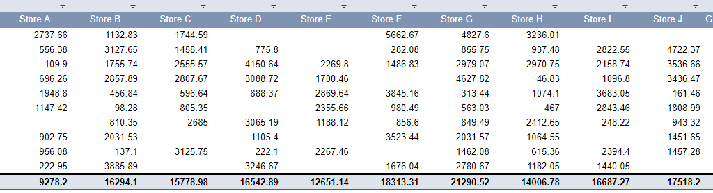
For this example, I’m going to use the following data for my pivot table:
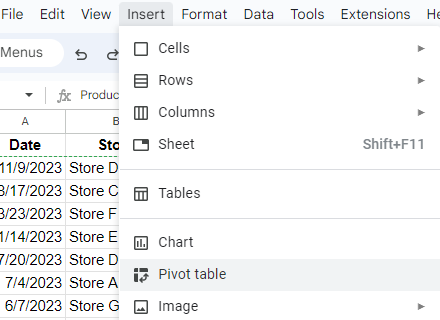
To create a pivot table with this range, all I need to do is, with a cell selected, to go to the Insert menu and click on Pivot Table
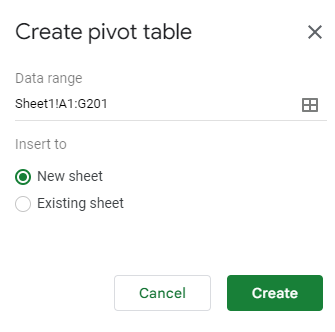
As long as you have a cell selected on your data set, Google Sheets will automatically detect your range. If it looks correct, you can just select whether you want it to be placed in a new sheet or an existing sheet, and then click on Create.
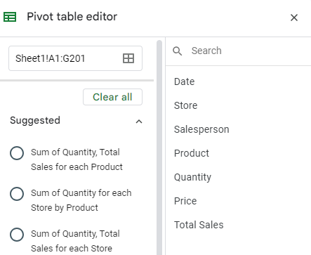
The next part is to setup the pivot table and ensure that the value section contains values and you have something in either the rows, columns, or filters sections to summarize your data. In my example, I’m going to summarize my data by rep and store:
The pivot table is setup but the problem is it won’t automatically update. Here’s how we can fix that.
Setting up your pivot table so that it automatically updates in Google Sheets
The problem with this pivot table lies with the range. While Google Sheets correctly detected a range, it also set it to a specific number of rows. My data set went up to row 201 as it contained 200 rows of data. But if I add more data, my pivot table won’t automatically expand. To get around this, I need to adjust my pivot table range.
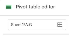
With my pivot table selected, I can see the range that it references in the Pivot table editor pane:
If I add another row of data, I can adjust this range so that it goes from A1:G202. But this would be a very tedious task if every time I added data I needed to remember to adjust the range. Instead, what I can do is adjust my range so that it references entire columns. By doing this, Google Sheets will automatically detect the size of my data set. In this example, I just need to set my range to A:G:
Now my pivot table will include a blank value under the Salesperson field as well as a blank store value.
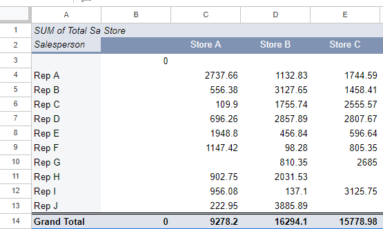
To fix this, what I can do is hide row 3 and column B, since these ranges contain the blanks. And as long as the blank values always appear first, this can be an effective way to hide the data, even if the pivot table expands.
If you like this post on How to Create an Automatically Updating Pivot Table in Google Sheets, please give this site a like on Facebook and also be sure to check out some of the many templates that we have available for download. You can also follow me on Twitter and YouTube. Also, please consider buying me a coffee if you find my website helpful and would like to support it.