
If you want to create conditional formatting rules but want to easily change the cutoff values for them, you can link your rules to specific cells, to make that process easy. Below, I’ll show you how to make your conditional formatting rules dynamic. Rather than going into the settings each time, you can just update specific cells, which will change your cutoff points.
Creating conditional formatting rules for changes in stock prices
A common example where you might want to adjust the cutoff values for conditional formatting rules is when dealing with stock prices. Suppose you want to highlight stocks when they have risen by more than 5%. But in other cases, such as when you’re looking at a long time frame, you may want the threshold to be much higher than that. This is where linking conditional formatting rules can be advantageous, by making the update process easier.
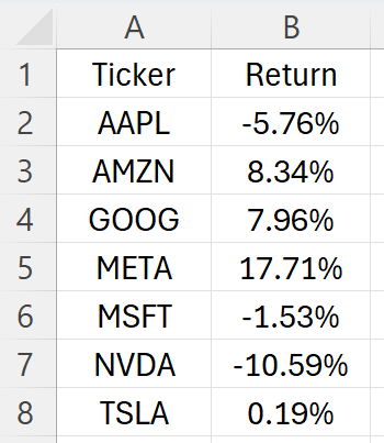
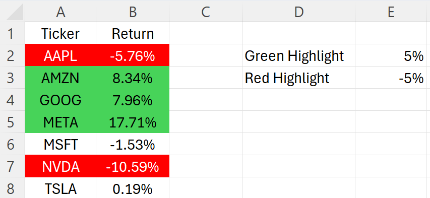
In the spreadsheet below, I have a list of stocks and their respective returns between December 31, 2024 and January 31, 2025. I have pulled in their performances using Excel’s STOCKHISTORY function.
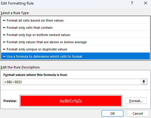
In this scenario, I may want to highlight stocks which have returns of more than 5% as green, and those which are down by 5% in red. I’ll create two conditional formatting rules to highlight both the return and the stock. Here’s how one of the rules looks:
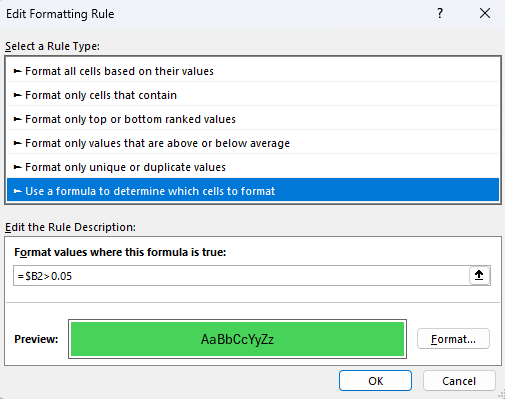
The downside of this rule is that the 0.05 value is hardcoded. If I want to change the threshold, I would need to go back into the conditional formatting rules and modify it. There is an easier way around this, and that’s by just linking to a specific cell.
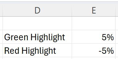
In the above example, I’ve entered the values that I want to link my conditional formatting rules to. In the case of a green highlight, I’m going to link to cell E2. And when I’m formatting the cells red, I’ll link to cell E3. Here’s how my updated conditional formatting rule will look:

Now, I’ve removed the hardcoded value and my conditional formatting rule now points to a specific cell, which is frozen and doesn’t change. To do the same thing for my red highlight rule, when the values are down 5%, I do the same thing, except flip the sign and refer to cell $E$3:
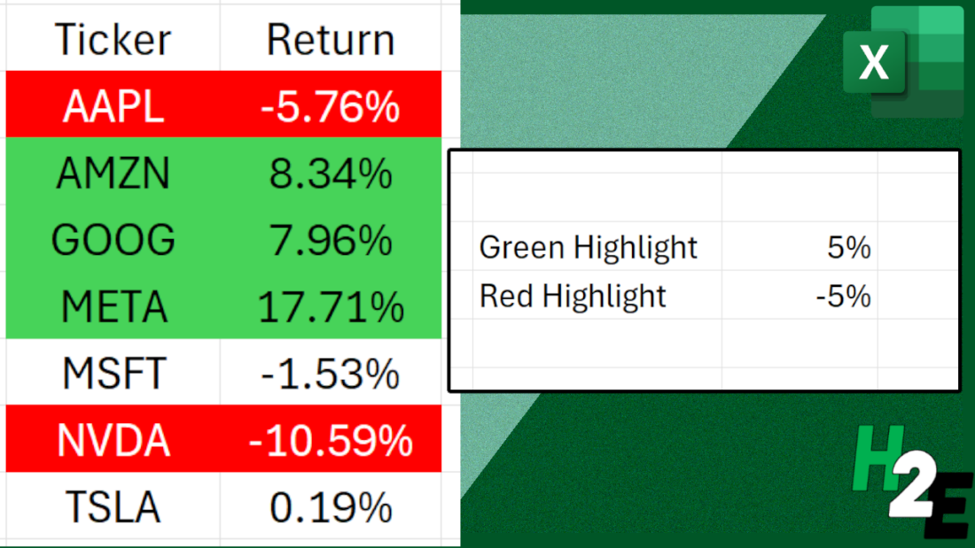
My conditional formatting rules are correctly applied to my data set, highlighting returns of more than 5% in green, and returns of less than negative 5% in red:
The advantage here is I can easily update my thresholds by just modifying the values in column E. If I change them to 10% for green and -10% for red, I simply make the changes in those cells and my conditional formatting updates immediately:
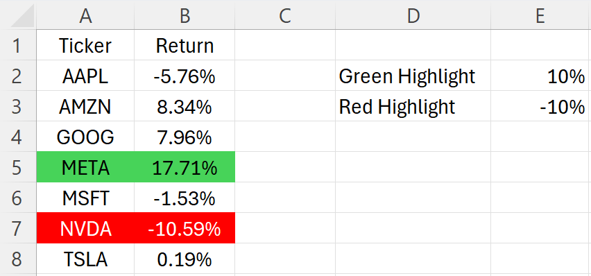
By setting up my conditional formatting rules this way, it’s easy to update the process in seconds and at the same time, I can see what my threshold are.
If you like this post on How to Apply Dynamic Conditional Formatting and Link Rules to Specific Cells, please give this site a like on Facebook and also be sure to check out some of the many templates that we have available for download. You can also follow me on Twitter and YouTube. Also, please consider buying me a coffee if you find my website helpful and would like to support it.